Arrays#
![]()

Note
If you have the basic knowledge about NumPy (the array here is the same as the ndarray in NumPy), you can skip this section.
In this section, we are going to understand:
What is a
array?How to create a
array?What operations are supported for a
array?
import brainpy.math as bm

bm.set_platform('cpu')
What is array?#
A array is a homogeneous multidimensional array. It is a table of elements (usually numbers), all of the same type, indexed by a tuple of non-negative integers. The dimensions of an array are called axes.
In the following picture, the 1D array ([7, 2, 9, 10]) only has one axis. There are 4 elements in this axis, so the shape of the array is (4,).
By contrast, the 2D array
[[5.2, 3.0, 4.5],
 [9.1, 0.1, 0.3]]
has 2 axes. The first axis has a length of 2 and the second has a length of 3. Therefore, the shape of the 2D array is (2, 3).
Similarly, the 3D array has 3 axes, with the dimensions (4, 3, 2) in each axis, respectively.

A array has several important attributes:
.ndim: the number of axes (dimensions) of the array.
.shape: the dimensions of the array. This is a tuple of integers indicating the size of the array in each dimension. For a matrix with n rows and m columns, the shape will be
(n,m). The length of the shape tuple is therefore the number of axes,ndim..size: the total number of elements of the array. This is equal to the product of the elements of shape.
.dtype: an object describing the type of the elements in the array. One can create or specify dtypes using standard Python types.
a = bm.arange(15).reshape((3, 5))

a
JaxArray(DeviceArray([[ 0,  1,  2,  3,  4],
                      [ 5,  6,  7,  8,  9],
                      [10, 11, 12, 13, 14]], dtype=int32))
a.shape
(3, 5)
a.ndim
2
a.dtype
dtype('int32')
How to create a array?#
There are several ways to create a array.
1. array(), zeros() and ones()#
The basic method is to convert Python sequences into arrays by bm.array(). For example:
bm.array([2, 3, 4])
JaxArray(DeviceArray([2, 3, 4], dtype=int32))
bm.array([(1.5, 2, 3), (4, 5, 6)])
JaxArray(DeviceArray([[1.5, 2. , 3. ],
                      [4. , 5. , 6. ]], dtype=float32))
Often, the elements of an array are originally unknown, but its size is known. Therefore, you can use placeholder functions to create arrays, like:
# "bm.zeros()" creates an array full of zeros

bm.zeros((3, 4))
JaxArray(DeviceArray([[0., 0., 0., 0.],
                      [0., 0., 0., 0.],
                      [0., 0., 0., 0.]], dtype=float32))
# "bm.ones()" creates an array full of ones

bm.ones((3, 4))
JaxArray(DeviceArray([[1., 1., 1., 1.],
                      [1., 1., 1., 1.],
                      [1., 1., 1., 1.]], dtype=float32))
2. linspace() and arange()#
Another two commonly used 1D array creation functions are bm.linspace() and bm.arange().
bm.arange() creates arrays with regularly incrementing values. It receives “start”, “end”, and “step” settings.
# if only one argument "A" are provided, the function will
# recognize the "start = 0", "end = A", and "step = 1" .

bm.arange(10)
JaxArray(DeviceArray([0, 1, 2, 3, 4, 5, 6, 7, 8, 9], dtype=int32))
# if two argument "A, B" are provided, the function will
# recognize the "start = A", "end = B", and "step = 1" .

bm.arange(2, 10, dtype=float)
JaxArray(DeviceArray([2., 3., 4., 5., 6., 7., 8., 9.], dtype=float32))
# if three argument "A, B, C" are provided, the function will
# recognize the "start = A", "end = B", and "step = C" .

bm.arange(2, 3, 0.1)
JaxArray(DeviceArray([2.       , 2.1      , 2.1999998, 2.2999997, 2.3999996,
                      2.4999995, 2.5999994, 2.6999993, 2.7999992, 2.8999991],            dtype=float32))
Due to the finite floating-point precision, it is generally impossible to predict the number of elements obtained by bm.arange(). For this reason, it is usually better to use the function bm.linspace() that receives “start”, “end”, and “num” settings.
bm.linspace(2, 3, 10)
JaxArray(DeviceArray([2.       , 2.1111112, 2.2222223, 2.3333333, 2.4444447,
                      2.5555556, 2.6666665, 2.777778 , 2.8888888, 3.       ],            dtype=float32))
3. Random sampling#
brainpy.math module provides convenient random sampling functions. This module contains some simple random data generation methods, some permutation and distribution functions, and random generator functions. Here I just give several examples.
brainpy.math.random.rand(d0, d1, ..., dn)
This function of random module is used to generate random numbers or values in a given shape.
bm.random.rand(5, 2)
JaxArray(DeviceArray([[0.07216692, 0.2877245 ],
                      [0.29642737, 0.43941212],
                      [0.9228879 , 0.14709306],
                      [0.8345591 , 0.8134085 ],
                      [0.6776234 , 0.42747045]], dtype=float32))
brainpy.math.random.randn(d0, d1, ..., dn)
This function of random module returns a sample from the “standard normal” distribution.
bm.random.randn(5, 2)
JaxArray(DeviceArray([[-1.2456564 ,  0.93986976],
                      [ 1.2722825 , -0.5604058 ],
                      [ 0.42648995,  1.2291526 ],
                      [ 0.7283678 ,  0.12521066],
                      [ 0.29101485,  2.0382316 ]], dtype=float32))
brainpy.math.random.randint(low, high[, size, dtype])
This function of random module is used to generate random integers from inclusive(low) to exclusive(high).
bm.random.randint(0, 3, size=10)
JaxArray(DeviceArray([0, 0, 0, 1, 2, 0, 1, 1, 1, 1], dtype=int32))
brainpy.math.random.random([size])
This function of random module is used to generate random floats number in the half-open interval [0.0, 1.0).
bm.random.random((3, 2))
JaxArray(DeviceArray([[0.30104673, 0.08174968],
                      [0.46729672, 0.30544508],
                      [0.37684703, 0.7211865 ]], dtype=float32))
brainpy.math module also provides permutation functions.
brainpy.math.random.shuffle()
This function is used to modify a sequence in-place by shuffling its contents.
bm.random.shuffle( bm.arange(10) )
JaxArray(DeviceArray([5, 9, 4, 0, 3, 2, 6, 8, 7, 1], dtype=int32))
brainpy.math.random.permutation()
This function permute a sequence randomly or return a permuted range.
bm.random.permutation( bm.arange(10) )
JaxArray(DeviceArray([1, 4, 8, 5, 2, 7, 3, 9, 0, 6], dtype=int32))
brainpy.math module also provides functions to sample distributions.
beta(a, b[, size])
This function is used to draw samples from a Beta distribution.
bm.random.beta(2, 3, 10)
JaxArray(DeviceArray([0.5404635 , 0.5812938 , 0.22380598, 0.20873289, 0.5460086 ,
                      0.11106081, 0.69154614, 0.28446677, 0.24081689, 0.6313805 ],            dtype=float32))
exponential([scale, size])
This function is used to draw sample from an exponential distribution.
bm.random.exponential(1, 10)
JaxArray(DeviceArray([0.828246  , 0.21370666, 0.32322478, 1.7631028 , 2.4889555 ,
                      1.133313  , 0.37169302, 0.32336047, 0.34985116, 0.2314292 ],            dtype=float32))
More sampling methods please see random sampling functions.
4. Other methods#
Moreover, there are many other methods we can use to create arrays, including:
Conversion from other Python structures (i.e. lists and tuples)
Intrinsic NumPy array creation functions (e.g.
arange,ones,zeros, etc.)Use of special library functions (e.g.,
random)Replicating, joining, or mutating existing arrays
Reading arrays from disk, either from standard or custom formats
Creating arrays from raw bytes through the use of strings or buffers
For details of these methods, please see NumPy tutorial: Array creation. Most of these methods are supported in BrainPy.
Supported operations on array#
All the operations in BrainPy are based on arrays. Therefore it is necessary to know what operations supported in each array object.
Basic operations#
Arithmetic operators on arrays apply element-wise. Let’s take “+”, “-”, “*”, and “/” as examples.
We first create two arrays:
data = bm.array([1, 2])

data
JaxArray(DeviceArray([1, 2], dtype=int32))
ones = bm.ones(2)

ones
JaxArray(DeviceArray([1., 1.], dtype=float32))

data + ones
JaxArray(DeviceArray([2., 3.], dtype=float32))

data - ones
JaxArray(DeviceArray([0., 1.], dtype=float32))
data * data
JaxArray(DeviceArray([1, 4], dtype=int32))
data / data
JaxArray(DeviceArray([1., 1.], dtype=float32))

Aggregation functions can also be performed on arrays, like:
.min(): to get the minimum element;.max(): to get the maximum element;.sum(): to get the summation;.mean(): to get the average;.prod(): to get the result of multiplying the elements together;.std(): to get the standard deviation.
data = bm.array([1, 2, 3])

data.max()
DeviceArray(3, dtype=int32)
data.min()
DeviceArray(1, dtype=int32)
data.sum()
DeviceArray(6, dtype=int32)

It’s very common to specify the aggregation along a row or column. For example, you can find the maximum value within each column by specifying axis=0.
a = bm.array([[1, 2],
              [5, 3],
              [4, 6]])
a.max(axis=0)
JaxArray(DeviceArray([5, 6], dtype=int32))
a.max(axis=1)
JaxArray(DeviceArray([2, 5, 6], dtype=int32))

Broadcasting#
array operations are usually done on pairs of arrays on an element-by-element basis. In the simplest case, the two arrays must have exactly the same shape, as in the following example:
a = bm.array([1.0, 2.0, 3.0])
b = bm.array([2.0, 2.0, 2.0])

a * b
JaxArray(DeviceArray([2., 4., 6.], dtype=float32))
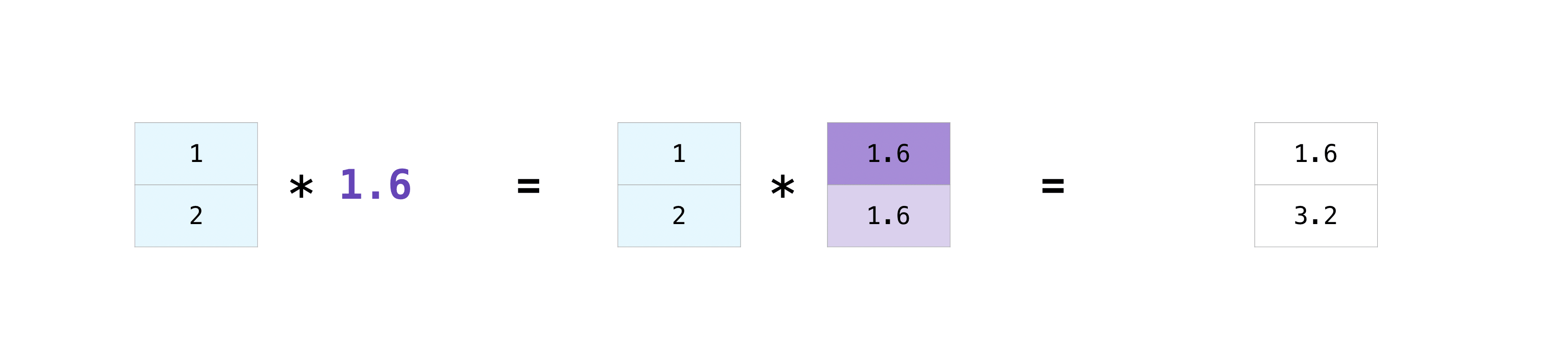
However, the broadcasting rule may be relaxed when the shapes of the arrays meet certain constraints. The simplest broadcasting example occurs when a array and a scalar value are combined in an operation:
a = bm.array([1, 2])
b = 1.6

a * b
JaxArray(DeviceArray([1.6, 3.2], dtype=float32, weak_type=True))
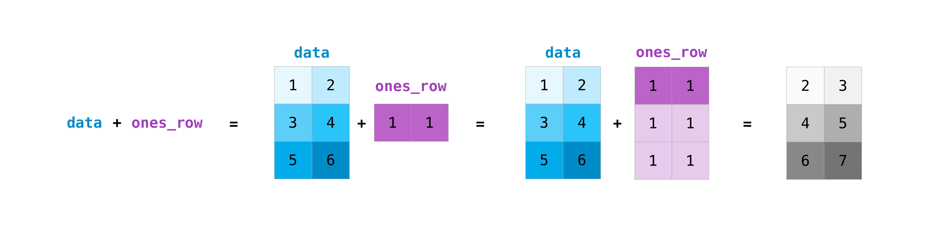
Similarly, broadcasting can be applied to matrices:
data = bm.array([[1, 2],
                 [3, 4],
                 [5, 6]])

ones_row = bm.array([[1, 1]])

data + ones_row
JaxArray(DeviceArray([[2, 3],
                      [4, 5],
                      [6, 7]], dtype=int32))
Under certain constraints, the smaller array can be “broadcast” across the larger array so that they have compatible shapes. Broadcasting provides a means of vectorizing array operations so that looping occurs in C instead of Python. It does this without making needless copies of data and usually leads to efficient algorithm implementations.
Generally, the dimensions of two arrays are compatible when
they are equal,
one of them is 1, or
one of them has fewer dimensions
If these conditions are not met, an error will occur.
For example, according to the broadcasting rules, the following two shapes are compatible:
Image  (3d array): 256 x 256 x 3
Scale  (1d array):             3
Result (3d array): 256 x 256 x 3
image = bm.random.random((256, 256, 3))
scale = bm.random.random(3)

_ = image + scale
_ = image - scale
_ = image * scale
_ = image / scale
These shapes are also compatible:
A      (4d array):  8 x 1 x 6 x 1
B      (3d array):      7 x 1 x 5
Result (4d array):  8 x 7 x 6 x 5
A = bm.random.random((8, 1, 6, 1))
B = bm.random.random((7, 1, 5))

_ = A + B
_ = A - B
_ = A * B
_ = A / B
However, in these examples, the shapes cannot be broadcast:
A      (1d array):  3
B      (1d array):  4 # trailing dimensions do not match

A      (2d array):      2 x 1
B      (3d array):  8 x 4 x 3 # second from last dimensions mismatched
A = bm.random.random((3,))
B = bm.random.random((4,))

try:
    _ = A + B
except Exception as e:
    print(e)
add got incompatible shapes for broadcasting: (3,), (4,).
A = bm.random.random((2, 1))
B = bm.random.random((8, 4, 3))

try:
    _ = A + B
except Exception as e:
    print(e)
Incompatible shapes for broadcasting: ((1, 2, 1), (8, 4, 3))
For more details about broadcasting, please see NumPy documentation: broadcasting.
Indexing, Slicing and Iterating#
arrays can be indexed, sliced, and iterated over, much like lists and other Python sequences. For examples:
a = bm.arange(10) ** 3

a
JaxArray(DeviceArray([ 0, 1, 8, 27, 64, 125, 216, 343, 512, 729], dtype=int32))
a[2]
DeviceArray(8, dtype=int32)
a[2:5]
DeviceArray([ 8, 27, 64], dtype=int32)
# from start to position 6, exclusive, set every 2nd element to 1000,
# equivalent to a[0:6:2] = 1000

a[:6:2] = 1000

a
JaxArray(DeviceArray([1000, 1, 1000, 27, 1000, 125, 216, 343, 512, 729], dtype=int32))
a[::-1] # reversed a
DeviceArray([ 729, 512, 343, 216, 125, 1000, 27, 1000, 1, 1000], dtype=int32)
for i in a:  # iterate a
    print(i**(1 / 3.))
10.000001
1.0
10.000001
3.0
10.000001
5.0000005
6.0000005
7.0000005
8.000001
9.000001
For multi-dimensional arrays, these indices should be given in a tuple separated by commas. For example:
b = bm.arange(20).reshape((5, 4))
b[2, 3]
DeviceArray(11, dtype=int32)
b[0:5, 1] # each row in the second column of b
DeviceArray([ 1, 5, 9, 13, 17], dtype=int32)
b[:, 1] # equivalent to the previous example
DeviceArray([ 1, 5, 9, 13, 17], dtype=int32)
b[1:3, :] # each column in the second and third row of b
DeviceArray([[ 4,  5,  6,  7],
             [ 8,  9, 10, 11]], dtype=int32)
When fewer indices are provided than the number of axes, the missing indices are considered complete slices:
b[-1] # the last row. Equivalent to b[-1, :]
DeviceArray([16, 17, 18, 19], dtype=int32)
You can also write this using dots as b[i, ...]. The dots (...) represent as many colons as needed to produce a complete indexing tuple. For example, if x is an array with 5 axes, then
x[1, 2, ...]is equivalent tox[1, 2, :, :, :],x[..., 3]tox[:, :, :, :, 3]andx[4, ..., 5, :]tox[4, :, :, 5, :].
c = bm.arange(48).reshape((6, 4, 2))
c[1, ...] # same as c[1, :, :] or c[1]
DeviceArray([[ 8,  9],
             [10, 11],
             [12, 13],
             [14, 15]], dtype=int32)
c[..., 1] # same as c[:, :, 1]
DeviceArray([[ 1,  3,  5,  7],
             [ 9, 11, 13, 15],
             [17, 19, 21, 23],
             [25, 27, 29, 31],
             [33, 35, 37, 39],
             [41, 43, 45, 47]], dtype=int32)
Iterating over multidimensional arrays is done with respect to the first axis:
for row in b:
    print(row)
[0 1 2 3]
[4 5 6 7]
[ 8  9 10 11]
[12 13 14 15]
[16 17 18 19]
For more methods or advanced indexing and index tricks, please see NumPy tutorial: Indexing.
Mathematical functions#
arrays support many other functions, including
and others.
Most of these functions can be found in brainpy.math module. Let’s take a look at trigonometric, hyperbolic, and rounding functions.
d = bm.linspace(0, 1, 10)

d
JaxArray(DeviceArray([0.        , 0.11111111, 0.22222222, 0.33333334, 0.44444445,
                      0.5555556 , 0.6666667 , 0.7777778 , 0.8888889 , 1.        ],            dtype=float32))
# trigonometric functions

bm.sin(d)
JaxArray(DeviceArray([0.        , 0.11088263, 0.22039774, 0.32719472, 0.42995638,
                      0.5274154 , 0.6183698 , 0.7016979 , 0.7763719 , 0.84147096],            dtype=float32))
bm.arcsin(d)
JaxArray(DeviceArray([0.        , 0.11134101, 0.2240931 , 0.3398369 , 0.460554  ,
                      0.58903104, 0.7297277 , 0.8911225 , 1.0949141 , 1.5707964 ],            dtype=float32))
# hyperbolic functions

bm.sinh(d)
JaxArray(DeviceArray([0.        , 0.11133985, 0.22405571, 0.33954054, 0.45922154,
                      0.58457786, 0.7171585 , 0.8586021 , 1.0106566 , 1.1752012 ],            dtype=float32))
# rounding functions

bm.round(d)
JaxArray(DeviceArray([0., 0., 0., 0., 0., 1., 1., 1., 1., 1.], dtype=float32))
# sum function

bm.sum(d)
DeviceArray(5., dtype=float32)