Building Network Models
Contents
Building Network Models#
In previous sections, it has been illustrated how to define neuron models by brainpy.dyn.NeuGroup and synapse models by brainpy.dyn.TwoEndConn. This section will introduce brainpy.dyn.Network, which is the base class used to build network models.
In essence, brainpy.dyn.Network is a container, whose function is to compose the individual elements. It is a subclass of a more general class: brainpy.dyn.Container.
In below, we take an excitation-inhibition (E-I) balanced network model as an example to illustrate how to compose the LIF neurons and Exponential synapses defined in previous tutorials to build a network.
import brainpy as bp

bp.math.set_platform('cpu')
Excitation-Inhibition (E-I) Balanced Network#
The E-I balanced network was first proposed to explain the irregular firing patterns of cortical neurons and comfirmed by experimental data. The network [1] we are going to implement consists of excitatory (E) neurons and inhibitory (I) neurons, the ratio of which is about 4 : 1. The biggest difference between excitatory and inhibitory neurons is the reversal potential - the reversal potential of inhibitory neurons is much lower than that of excitatory neurons. Besides, the membrane time constant of inhibitory neurons is longer than that of excitatory neurons, which indicates that inhibitory neurons have slower dynamics.
[1] Brette, R., Rudolph, M., Carnevale, T., Hines, M., Beeman, D., Bower, J. M., et al. (2007), Simulation of networks of spiking neurons: a review of tools and strategies., J. Comput. Neurosci., 23, 3, 349–98.
# BrianPy has some built-in conanical neuron and synapse models

LIF = bp.dyn.neurons.LIF
ExpCOBA = bp.dyn.synapses.ExpCOBA
Two ways to define network models#
There are several ways to define a Network model.
1. Defining a network as a class#
The first way to define a network model is like follows.
class EINet(bp.dyn.Network):
  def __init__(self, num_exc, num_inh, method='exp_auto', **kwargs):
    super(EINet, self).__init__(**kwargs)

    # neurons
    pars = dict(V_rest=-60., V_th=-50., V_reset=-60., tau=20., tau_ref=5.)
    E = LIF(num_exc, **pars, method=method)
    I = LIF(num_inh, **pars, method=method)
    E.V.value = bp.math.random.randn(num_exc) * 2 - 55.
    I.V.value = bp.math.random.randn(num_inh) * 2 - 55.

    # synapses
    w_e = 0.6  # excitatory synaptic weight
    w_i = 6.7  # inhibitory synaptic weight
    E_pars = dict(E=0., g_max=w_e, tau=5.)
    I_pars = dict(E=-80., g_max=w_i, tau=10.)

    # Neurons connect to each other randomly with a connection probability of 2%
    self.E2E = ExpCOBA(E, E, bp.conn.FixedProb(prob=0.02), **E_pars, method=method)
    self.E2I = ExpCOBA(E, I, bp.conn.FixedProb(prob=0.02), **E_pars, method=method)
    self.I2E = ExpCOBA(I, E, bp.conn.FixedProb(prob=0.02), **I_pars, method=method)
    self.I2I = ExpCOBA(I, I, bp.conn.FixedProb(prob=0.02), **I_pars, method=method)

    self.E = E
    self.I = I
In an instance of brainpy.dyn.Network, all self. accessed elements can be gathered by the .child_ds() function automatically.
EINet(8, 2).child_ds()
{'ExpCOBA0': <brainpy.dyn.synapses.abstract_models.ExpCOBA at 0x1076db580>,
 'ExpCOBA1': <brainpy.dyn.synapses.abstract_models.ExpCOBA at 0x1584c3d30>,
 'ExpCOBA2': <brainpy.dyn.synapses.abstract_models.ExpCOBA at 0x158496a00>,
 'ExpCOBA3': <brainpy.dyn.synapses.abstract_models.ExpCOBA at 0x15880ce80>,
 'LIF0': <brainpy.dyn.neurons.IF_models.LIF at 0x1583fd100>,
 'LIF1': <brainpy.dyn.neurons.IF_models.LIF at 0x1583f6d30>,
 'ConstantDelay0': <brainpy.dyn.base.ConstantDelay at 0x1584ba1c0>,
 'ConstantDelay1': <brainpy.dyn.base.ConstantDelay at 0x1584c3d00>,
 'ConstantDelay2': <brainpy.dyn.base.ConstantDelay at 0x158496370>,
 'ConstantDelay3': <brainpy.dyn.base.ConstantDelay at 0x15880c340>}
Note in the above EINet, we do not define the update() function. This is because any subclass of brainpy.dyn.Network has a default update function, in which it automatically gathers the elements defined in this network and sequentially runs the update function of each element.
If you have some special operations in your network, you can override the update function by yourself. Here is a simple example.
class ExampleToOverrideUpdate(EINet):
    def update(self, _t, _dt):
        for node in self.child_ds().values():
            node.update(_t, _dt)
Let’s try to simulate our defined EINet model.
net = EINet(3200, 800, method='exp_auto') # "method": the numerical integrator method
runner = bp.dyn.DSRunner(net,
monitors=['E.spike', 'I.spike'],
inputs=[('E.input', 20.), ('I.input', 20.)])
t = runner.run(100.)
print(f'Used time {t} s')
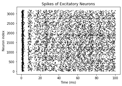
# visualization
bp.visualize.raster_plot(runner.mon.ts, runner.mon['E.spike'],
title='Spikes of Excitatory Neurons', show=True)
bp.visualize.raster_plot(runner.mon.ts, runner.mon['I.spike'],
title='Spikes of Inhibitory Neurons', show=True)
Used time 0.35350608825683594 s

2. Instantiating a network directly#
Another way to instantiate a network model is directly pass the elements into the constructor of brainpy.Network. It receives *args and **kwargs arguments.
# neurons
pars = dict(V_rest=-60., V_th=-50., V_reset=-60., tau=20., tau_ref=5.)
E = LIF(3200, **pars)
I = LIF(800, **pars)
E.V.value = bp.math.random.randn(E.num) * 2 - 55.
I.V.value = bp.math.random.randn(I.num) * 2 - 55.

# synapses
E_pars = dict(E=0., g_max=0.6, tau=5.)
I_pars = dict(E=-80., g_max=6.7, tau=10.)
E2E = ExpCOBA(E, E, bp.conn.FixedProb(prob=0.02), **E_pars)
E2I = ExpCOBA(E, I, bp.conn.FixedProb(prob=0.02), **E_pars)
I2E = ExpCOBA(I, E, bp.conn.FixedProb(prob=0.02), **I_pars)
I2I = ExpCOBA(I, I, bp.conn.FixedProb(prob=0.02), **I_pars)


# Network
net2 = bp.dyn.Network(E2E, E2I, I2E, I2I, exc_group=E, inh_group=I)
All elements are passed as **kwargs argument can be accessed by the provided keys. This will affect the following dynamics simualtion and will be discussed in greater detail in tutorial of Runners.
net2.exc_group
<brainpy.dyn.neurons.IF_models.LIF at 0x159470c10>
net2.inh_group
<brainpy.dyn.neurons.IF_models.LIF at 0x159470d30>
After construction, the simulation goes the same way:
runner = bp.dyn.DSRunner(net2,
                         monitors=['exc_group.spike', 'inh_group.spike'],
                         inputs=[('exc_group.input', 20.), ('inh_group.input', 20.)])
t = runner.run(100.)
print(f'Used time {t} s')

# visualization
bp.visualize.raster_plot(runner.mon.ts, runner.mon['exc_group.spike'],
                         title='Spikes of Excitatory Neurons', show=True)
bp.visualize.raster_plot(runner.mon.ts, runner.mon['inh_group.spike'],
                         title='Spikes of Inhibitory Neurons', show=True)
Used time 0.3590219020843506 s


Above are some simulation examples showing the possible application of network models. The detailed description of dynamics simulation is covered in the toolboxes, where the use of runners, monitors, and inputs will be expatiated.