Training a Brain Dynamics Model

@Chaoming Wang

In recent years, we saw the revolution that training a dynamical system from data or tasks has provided important insights to understand brain functions. To support this, BrainPy provides various interfaces to help users train dynamical systems.

import brainpy as bp
import brainpy.math as bm
import brainpy_datasets as bd
import matplotlib.pyplot as plt

bm.enable_x64()

bm.set_platform('cpu')

bp.__version__

'3.0.0'

Training a reservoir network model

For an echo state network, we have three components: an input node (“I”), a reservoir node (“R”) for dimension expansion, and an output node (“O”) for linear readout.

(Gauthier, et. al., Nature Communications, 2021) has proposed a next generation reservoir computing (NG-RC) model by using nonlinear vector autoregression (NVAR).

The difference between the two models is illustrated in the following figure.

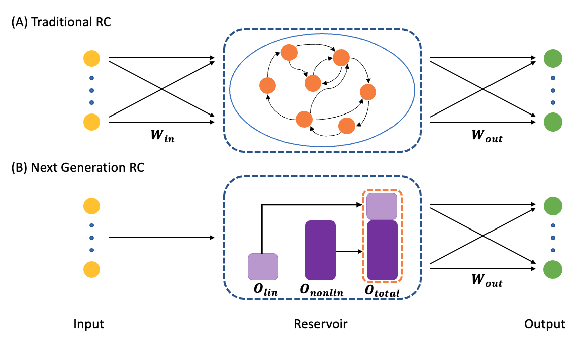
(A) A traditional RC processes time-series data using an artificial recurrent neural network. (B) The NG-RC performs a forecast using a linear weight of time-delay states of the time series data and nonlinear functionals of this data.

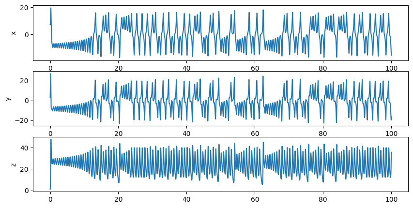
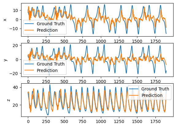
Here, let’s implement a next generation reservoir model to predict the chaotic time series, named as Lorenz attractor. Particularly, we expect the network has the ability to predict \(P(t+l)\) from \(P(t)\), where \(l\) is the length of the prediction ahead.

dt = 0.01
data = bd.chaos.LorenzEq(100, dt=dt)

plt.figure(figsize=(10, 5))
plt.subplot(311)
plt.plot(bm.as_numpy(data.ts), bm.as_numpy(data.xs.flatten()))
plt.ylabel('x')
plt.subplot(312)
plt.plot(bm.as_numpy(data.ts), bm.as_numpy(data.ys.flatten()))
plt.ylabel('y')
plt.subplot(313)
plt.plot(bm.as_numpy(data.ts), bm.as_numpy(data.zs.flatten()))
plt.ylabel('z')
plt.show()

Let’s first create a function to get the data.

def get_subset(data, start, end):
    res = {'x': data.xs[start: end],
           'y': data.ys[start: end],
           'z': data.zs[start: end]}
    res = bm.hstack([res['x'], res['y'], res['z']])
    return res.reshape((1, ) + res.shape)

To accomplish this task, we implement a next-generation reservoir model of 4 delay history information with stride of 5, and their quadratic polynomial monomials, same as (Gauthier, et. al., Nature Communications, 2021).

class NGRC(bp.DynamicalSystem):
  def __init__(self, num_in, num_out):
    super(NGRC, self).__init__()
    self.r = bp.dyn.NVAR(num_in, delay=4, order=2, stride=5)
    self.o = bp.dnn.Dense(self.r.num_out, num_out, mode=bm.training_mode)

  def update(self, x):
    return self.o(self.r(x))

with bm.environment(bm.batching_mode):  # Batching Computing Mode
    model = NGRC(num_in=3, num_out=3)

Moreover, we use Ridge Regression method to train the model.

trainer = bp.RidgeTrainer(model, alpha=1e-6)

We warm-up the network with 20 ms.

warmup_data = get_subset(data, 0, int(20/dt))

outs = trainer.predict(warmup_data)

# outputs should be an array with the shape of
# (num_batch, num_time, num_out)
outs.shape

(1, 2000, 3)

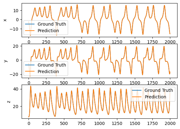
The training data is the time series from 20 ms to 80 ms. We want the network has the ability to forecast 1 time step ahead.

x_train = get_subset(data, int(20/dt), int(80/dt))
y_train = get_subset(data, int(20/dt)+1, int(80/dt)+1)

_ = trainer.fit([x_train, y_train])

Then we test the trained network with the next 20 ms.

x_test = get_subset(data, int(80/dt), int(100/dt)-1)
y_test = get_subset(data, int(80/dt) + 1, int(100/dt))

predictions = trainer.predict(x_test)

bp.losses.mean_squared_error(y_test, predictions)

Array(4.43051641e-09, dtype=float64)

def plot_difference(truths, predictions):
    truths = bm.as_numpy(truths)
    predictions = bm.as_numpy(predictions)

    plt.subplot(311)
    plt.plot(truths[0, :, 0], label='Ground Truth')
    plt.plot(predictions[0, :, 0], label='Prediction')
    plt.ylabel('x')
    plt.legend()
    plt.subplot(312)
    plt.plot(truths[0, :, 1], label='Ground Truth')
    plt.plot(predictions[0, :, 1], label='Prediction')
    plt.ylabel('y')
    plt.legend()
    plt.subplot(313)
    plt.plot(truths[0, :, 2], label='Ground Truth')
    plt.plot(predictions[0, :, 2], label='Prediction')
    plt.ylabel('z')
    plt.legend()
    plt.show()

plot_difference(y_test, predictions)

We can make the task harder to forecast 10 time step ahead.

warmup_data = get_subset(data, 0, int(20/dt))
outs = trainer.predict(warmup_data)

x_train = get_subset(data, int(20/dt), int(80/dt))
y_train = get_subset(data, int(20/dt)+10, int(80/dt)+10)
trainer.fit([x_train, y_train])

x_test = get_subset(data, int(80/dt), int(100/dt)-10)
y_test = get_subset(data, int(80/dt) + 10, int(100/dt))
predictions = trainer.predict(x_test)

plot_difference(y_test, predictions)

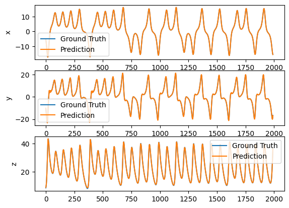
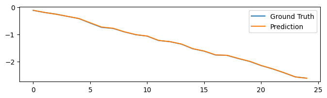
Or forecast 100 time step ahead.

warmup_data = get_subset(data, 0, int(20/dt))
_ = trainer.predict(warmup_data)

x_train = get_subset(data, int(20/dt), int(80/dt))
y_train = get_subset(data, int(20/dt)+100, int(80/dt)+100)
trainer.fit([x_train, y_train])

x_test = get_subset(data, int(80/dt), int(100/dt)-100)
y_test = get_subset(data, int(80/dt) + 100, int(100/dt))
predictions = trainer.predict(x_test)

plot_difference(y_test, predictions)

As you see, forecasting larger time step makes the learning more difficult.

Training an artificial recurrent network

In recent years, artificial recurrent neural networks trained with back propagation through time (BPTT) have been a useful tool to study the network mechanism of brain functions. To support training networks with BPTT, BrainPy provides brainpy.train.BPTT interface.

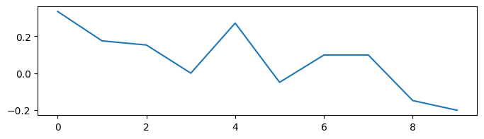
Here, we demonstrate how to train an artificial recurrent neural network by using a white noise integration task. In this task, we want our trained RNN model has the ability to integrate white noise. For example, if we have a time series of noise data,

noises = bm.random.normal(0, 0.2, size=10)

plt.figure(figsize=(8, 2))
plt.plot(noises.flatten())
plt.show()

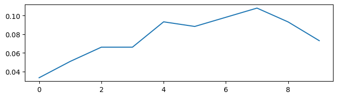
Now, we want to get a model which can integrate the noise bm.cumsum(noises) * dt:

dt = 0.1
integrals = bm.cumsum(noises) * dt

plt.figure(figsize=(8, 2))
plt.plot(integrals.flatten())
plt.show()

Here, we first define a task which generates the input data and the target integration results.

from functools import partial

dt = 0.04
num_step = int(1.0 / dt)
num_batch = 128


@bm.jit
def build_inputs_and_targets(mean=0.025, scale=0.01):
  # Create the white noise input
  sample = bm.random.normal(size=(num_batch, 1, 1))
  bias = mean * 2.0 * (sample - 0.5)
  samples = bm.random.normal(size=(num_batch, num_step, 1))
  noise_t = scale / dt ** 0.5 * samples
  inputs = bias + noise_t
  targets = bm.cumsum(inputs, axis=1)
  return inputs, targets


def train_data():
  for _ in range(100):
    yield build_inputs_and_targets()

Then, we create and initialize the model. Note here we need the model train its initial state, so we need set state_trainable=True for the used VanillaRNN instance.

class RNN(bp.DynamicalSystem):
  def __init__(self, num_in, num_hidden):
    super(RNN, self).__init__()
    self.rnn = bp.dyn.RNNCell(num_in, num_hidden, train_state=True)
    self.out = bp.dnn.Dense(num_hidden, 1)

  def update(self, x):
    return self.out(self.rnn(x))


with bm.training_environment():
    model = RNN(1, 100)

brainpy.nn.BPTT trainer receives a loss function setting, and an optimizer setting. Loss function can be selected from the brainpy.losses module, or it can be a callable function receives (predictions, targets) argument. Optimizer setting must be an instance of brainpy.optim.Optimizer.

Here we define a loss function which use Mean Squared Error (MSE) to measure the error between the targets and the predictions. We also apply a L2 regularization.

# define loss function
def loss(predictions, targets, l2_reg=2e-4):
    mse = bp.losses.mean_squared_error(predictions, targets)
    l2 = l2_reg * bp.losses.l2_norm(model.train_vars().unique().dict()) ** 2
    return mse + l2

# define optimizer
lr = bp.optim.ExponentialDecay(lr=0.025, decay_steps=1, decay_rate=0.99975)
opt = bp.optim.Adam(lr=lr, eps=1e-1)

D:\codes\projects\BrainPy\brainpy\version2\optim\scheduler.py:355: UserWarning: ExponentialDecay is abandoned, please use ExponentialDecayLR insteadly.
  warnings.warn("ExponentialDecay is abandoned, please use ExponentialDecayLR insteadly.")

# create a trainer
trainer = bp.BPTT(model, loss_fun=loss, optimizer=opt)

# train the model
trainer.fit(train_data, num_epoch=30)

Train 0 epoch, use 4.6525 s, loss 0.5769001624120187
Train 1 epoch, use 3.9341 s, loss 0.6012456617375284
Train 2 epoch, use 3.8690 s, loss 0.16763342151665736
Train 3 epoch, use 3.8010 s, loss 0.03367445910900796
Train 4 epoch, use 3.6578 s, loss 0.02507292572843596
Train 5 epoch, use 3.6672 s, loss 0.023660240621885324
Train 6 epoch, use 3.5259 s, loss 0.023234681320259867
Train 7 epoch, use 3.6066 s, loss 0.02274668271018847
Train 8 epoch, use 3.5556 s, loss 0.022179079240538725
Train 9 epoch, use 3.5196 s, loss 0.022273897407273986
Train 10 epoch, use 3.5467 s, loss 0.021910333591299028
Train 11 epoch, use 3.7714 s, loss 0.022207959184164894
Train 12 epoch, use 3.7795 s, loss 0.021711869384784855
Train 13 epoch, use 3.8430 s, loss 0.021634918551652463
Train 14 epoch, use 4.6484 s, loss 0.021597238429818838
Train 15 epoch, use 4.1485 s, loss 0.02158446679037941
Train 16 epoch, use 4.0141 s, loss 0.02143738330785308
Train 17 epoch, use 3.6024 s, loss 0.02147022388760562
Train 18 epoch, use 4.0315 s, loss 0.021425177991256376
Train 19 epoch, use 3.5877 s, loss 0.021317941077372508
Train 20 epoch, use 3.6267 s, loss 0.021166253611346927
Train 21 epoch, use 3.5071 s, loss 0.021217574957937285
Train 22 epoch, use 3.4340 s, loss 0.021064762943911866
Train 23 epoch, use 3.5373 s, loss 0.021120882311109722
Train 24 epoch, use 3.5057 s, loss 0.021049819783330124
Train 25 epoch, use 3.4965 s, loss 0.02103106952961301
Train 26 epoch, use 3.2875 s, loss 0.02095386507792798
Train 27 epoch, use 3.4473 s, loss 0.02087706482808289
Train 28 epoch, use 3.3152 s, loss 0.02084544251948843
Train 29 epoch, use 3.5087 s, loss 0.02083820570207805

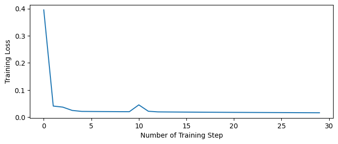
The training losses can be retrieved by .get_hist_metric() function.

plt.figure(figsize=(8, 3))
plt.plot(trainer.get_hist_metric(metric='loss'))
plt.xlabel('Number of Training Step')
plt.ylabel('Training Loss')
plt.show()

Finally, let’s try the trained network, and test whether it can generate the correct integration results.

model.reset(num_batch)
x, y = build_inputs_and_targets()
predicts = trainer.predict(x)

plt.figure(figsize=(8, 2))
plt.plot(bm.as_numpy(y[0]).flatten(), label='Ground Truth')
plt.plot(bm.as_numpy(predicts[0]).flatten(), label='Prediction')
plt.legend()
plt.show()

Training a spiking neural network

BrainPy also supports to train spiking neural networks.

In the following, we demonstrate how to use back-propagation algorithms to train spiking neurons with a simple example.

Our model is a simple three layer model:

• an input layer

• a LIF layer

• a readout layer

The synaptic connection between each layer is the Exponenetial synapse model.

bm.set_dt(1.)

class SNN(bp.DynamicalSystem):
  def __init__(self, num_in, num_rec, num_out):
    super().__init__()

    # parameters
    self.num_in = num_in
    self.num_rec = num_rec
    self.num_out = num_out

    # neuron groups
    self.r = bp.dyn.Lif(num_rec, tau=10., V_reset=0., V_rest=0., V_th=1.)
    self.o = bp.dyn.Integrator(num_out, tau=5.)

    # synapse: i->r
    self.i2r = bp.Sequential(
        comm=bp.dnn.Linear(num_in, num_rec, W_initializer=bp.init.KaimingNormal(scale=20.)),
        syn=bp.dyn.Expon(num_rec, tau=10.),
    )

    # synapse: r->o
    self.r2o = bp.Sequential(
        comm=bp.dnn.Linear(num_rec, num_out, W_initializer=bp.init.KaimingNormal(scale=20.)),
        syn=bp.dyn.Expon(num_out, tau=10.),
    )

  def update(self, spike):
    return spike >> self.i2r >> self.r >> self.r2o >> self.o

num_in = 100
num_rec = 10

with bm.training_environment():
    net = SNN(num_in, num_rec, 2)  # out task is a two label classification task

We try to use this simple task to classify a random spiking data into two classes.

num_step = 100
num_sample = 256
freq = 10  # Hz
mask = bm.random.rand(num_step, num_sample, num_in)
x_data = bm.zeros((num_step, num_sample, num_in))
x_data[mask < freq * bm.get_dt() / 1000.] = 1.0
y_data = bm.asarray(bm.random.rand(num_sample) < 0.5, dtype=bm.float_)
indices = bm.arange(num_step)

Same as the training of artificial recurrent neural networks, we use Adam optimizer and cross entropy loss to train the model.

class Trainer:
  def __init__(self, net, opt):
    self.net = net
    self.opt = opt
    opt.register_train_vars(net.train_vars().unique())
    self.f_grad = bm.grad(self.f_loss, grad_vars=self.opt.vars_to_train, return_value=True)

  def f_loss(self):
    self.net.reset(num_sample)
    outs = bm.for_loop(self.net.step_run, (indices, x_data))
    return bp.losses.cross_entropy_loss(bm.max(outs, axis=0), y_data)

  @bm.cls_jit
  def f_train(self):
    grads, loss = self.f_grad()
    self.opt.update(grads)
    return loss

trainer = Trainer(net=net, opt=bp.optim.Adam(lr=4e-3))
for i in range(1000):
  l = trainer.f_train()
  if (i + 1) % 100 == 0:
    print(f'Train {i + 1} steps, loss {l}')

Train 100 steps, loss 0.5695487842565937
Train 200 steps, loss 0.3587859591475745
Train 300 steps, loss 0.25472953093765993
Train 400 steps, loss 0.17916637832751206
Train 500 steps, loss 0.13153954348807992
Train 600 steps, loss 0.10446392929010859
Train 700 steps, loss 0.08519861963025842
Train 800 steps, loss 0.05897088855100058
Train 900 steps, loss 0.045521742857781
Train 1000 steps, loss 0.03488914109026672

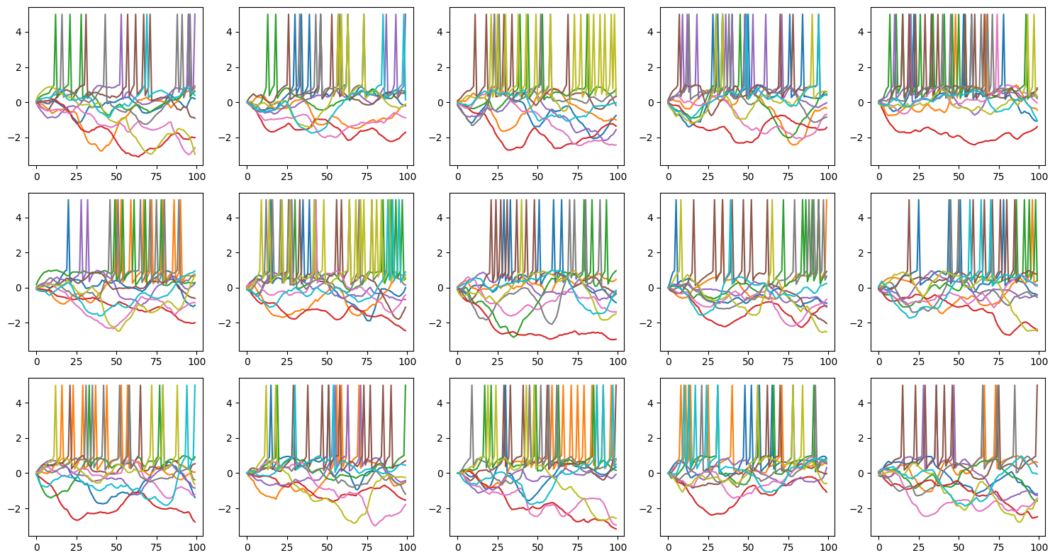
Let’s visualize the trained spiking neurons.

import numpy as np
from matplotlib.gridspec import GridSpec

def plot_voltage_traces(mem, spk=None, dim=(3, 5), spike_height=5):
  plt.figure(figsize=(15, 8))
  gs = GridSpec(*dim)
  mem = 1. * mem
  if spk is not None:
    mem[spk > 0.0] = spike_height
  mem = bm.as_numpy(mem)
  for i in range(np.prod(dim)):
    if i == 0:
      a0 = ax = plt.subplot(gs[i])
    else:
      ax = plt.subplot(gs[i], sharey=a0)
    ax.plot(mem[:, i])
  plt.tight_layout()
  plt.show()

runner = bp.DSRunner(
  net, data_first_axis='T',
  monitors={'r.spike': net.r.spike, 'r.membrane': net.r.V},
)
out = runner.run(inputs=x_data, reset_state=True)
plot_voltage_traces(runner.mon.get('r.membrane'), runner.mon.get('r.spike'))

# the prediction accuracy
m = bm.max(out, axis=0)  # max over time
am = bm.argmax(m, axis=1)  # argmax over output units
acc = bm.mean(y_data == am)  # compare to labels
print("Accuracy %.3f" % acc)

Accuracy 1.000