brainpy.neurons.PinskyRinzelModel

class brainpy.neurons.PinskyRinzelModel(size, keep_size=False, gNa=30.0, gK=15.0, gCa=10.0, gAHP=0.8, gC=15.0, gL=0.1, ENa=60.0, EK=-75.0, ECa=80.0, EL=-60.0, gc=2.1, V_th=20.0, Cm=3.0, p=0.5, A=1.0, Vs_initializer=OneInit(value=-64.6), Vd_initializer=OneInit(value=-64.5), Ca_initializer=OneInit(value=0.2), noise=None, method='exp_auto', name=None, mode=None)

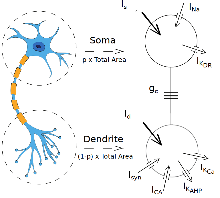
The Pinsky and Rinsel (1994) model.

The Pinsky and Rinsel (1994) model [7] is a 2-compartment (soma and dendrite), conductance-based (Hodgin-Huxley type) model of a hippocampal CA3 pyramidal neuron. It is a reduced version of an earlier, 19-compartment model by Traub, et. al. (1991) [8]. This model demonstrates how similar qualitative and quantitative spiking behaviors can be obtained despite the reduction in model complexity.

Specifically, this model demonstrates calcium bursting behavior and how the ‘ping-pong’ interplay between somatic and dendritic currents results in a complex shape of the burst.

Mathematically, the model is given by:

\[\begin{split} \begin{aligned} &\mathrm{C}_{\mathrm{m}} \mathrm{V}_{\mathrm{s}}^{\prime}=-\mathrm{I}_{\mathrm{Leak}}-\mathrm{I}_{\mathrm{Na}}-\mathrm{I}_{\mathrm{K}_{\mathrm{DR}}}-\frac{\mathrm{I}_{\mathrm{DS}}}{\mathrm{p}}+\frac{\mathrm{I}_{\mathrm{S}_{\mathrm{app}}}}{\mathrm{p}} \\ &\mathrm{C}_{\mathrm{m}} \mathrm{V}_{\mathrm{d}}^{\prime}=-\mathrm{I}_{\mathrm{Leak}}-\mathrm{I}_{\mathrm{Ca}}-\mathrm{I}_{\mathrm{K}_{\mathrm{Ca}}}-\mathrm{I}_{\mathrm{K}_{\mathrm{AHP}}}+\frac{\mathrm{I}_{\mathrm{SD}}}{(1-\mathrm{p})}+\frac{\mathrm{I}_{\mathrm{D}_{\mathrm{app}}}}{(1-\mathrm{p})} \\ &\frac{\mathrm{dCa}}{\mathrm{dt}}=-0.13 \mathrm{I}_{\mathrm{Ca}}-0.075 \mathrm{Ca} \end{aligned}\end{split}\]

The currents of the model are functions of potentials as follows:

\[\begin{split}\begin{aligned} \mathrm{I}_{\mathrm{Na}} &=\mathrm{g}_{\mathrm{Na}} m_{\infty}^{2}\left(\mathrm{~V}_{\mathrm{s}}\right) h\left(\mathrm{~V}_{\mathrm{s}}-\mathrm{V}_{\mathrm{Na}}\right) \\ \mathrm{I}_{\mathrm{K}_{\mathrm{DR}}} &=\mathrm{g}_{\mathrm{K}_{\mathrm{DR}}} n\left(\mathrm{~V}_{\mathrm{s}}-\mathrm{V}_{\mathrm{K}}\right) \\ \mathrm{I}_{\mathrm{Ca}} &=\mathrm{g}_{\mathrm{Ca}}{ }^{2}\left(\mathrm{~V}_{\mathrm{d}}-\mathrm{V}_{\mathrm{N}}\right) \\ \mathrm{I}_{\mathrm{K}_{\mathrm{Ca}}} &=\mathrm{g}_{\mathrm{k}_{\mathrm{Ca}}} C \chi(\mathrm{Ca})\left(\mathrm{V}_{\mathrm{d}}-\mathrm{V}_{\mathrm{Ca}}\right) \\ \mathrm{I}_{\mathrm{K}_{\mathrm{AHP}}} &=\mathrm{g}_{\mathrm{K}_{\mathrm{AHP}}} q\left(\mathrm{~V}_{\mathrm{d}}-\mathrm{V}_{\mathrm{K}}\right) \\ \mathrm{I}_{\mathrm{SD}} &=-\mathrm{I}_{\mathrm{DS}}=\mathrm{g}_{\mathrm{c}}\left(\mathrm{V}_{\mathrm{d}}-\mathrm{V}_{\mathrm{s}}\right) \\ \mathrm{I}_{\mathrm{Leak}} &=\mathrm{g}_{\mathrm{L}}\left(\mathrm{V}-\mathrm{V}_{\mathrm{L}}\right) \end{aligned}\end{split}\]

The activation and inactivation variables should satisfy these equations

\[\begin{split} \begin{aligned} \omega^{\prime}(\mathrm{V}) &=\frac{\omega_{\infty}(\mathrm{V})-\omega}{\tau_{\omega}(\mathrm{V})} \\ \omega_{\infty}(\mathrm{V}) &=\frac{\alpha_{\omega}(\mathrm{V})}{\alpha_{\omega}(\mathrm{V})+\beta_{\omega}(\mathrm{V})} \\ \tau_{\omega}(\mathrm{V}) &=\frac{1}{\alpha_{\omega}(\mathrm{V})+\beta_{\omega}(\mathrm{V})} \end{aligned}\end{split}\]

where, independently, we consider \(\omega = h, n, s, m, c, q\).

The rate functions are defined as follows

\[\begin{split} \begin{aligned} \alpha_{m}\left(\mathrm{~V}_{\mathrm{s}}\right) &=\frac{0.32\left(-46.9-\mathrm{V}_{\mathrm{s}}\right)}{\exp \left(\frac{-46.9-\mathrm{V}_{\mathrm{s}}}{4}\right)-1} \\ \beta_{m}\left(\mathrm{~V}_{\mathrm{s}}\right) &=\frac{0.28\left(\mathrm{~V}_{\mathrm{s}}+19.9\right)}{\exp \left(\frac{\mathrm{V}_{\mathrm{s}}+19.9}{5}\right)-1}, \\ \alpha_{n}\left(\mathrm{~V}_{\mathrm{s}}\right) &=\frac{0.016\left(-24.9-\mathrm{V}_{\mathrm{s}}\right)}{\exp \left(\frac{-24.9-\mathrm{V}_{\mathrm{s}}}{5}\right)-1} \\ \beta_{n}\left(\mathrm{~V}_{\mathrm{s}}\right) &=0.25 \exp \left(-1-0.025 \mathrm{~V}_{\mathrm{s}}\right) \\ \alpha_{h}\left(\mathrm{~V}_{\mathrm{s}}\right) &=0.128 \exp \left(\frac{-43-\mathrm{V}_{\mathrm{s}}}{18}\right) \\ \beta_{h}\left(\mathrm{~V}_{\mathrm{s}}\right) &=\frac{4}{1+\exp \left(\frac{\left(-20-\mathrm{V}_{\mathrm{s}}\right.}{5}\right)}, \\ \alpha_{s}\left(\mathrm{~V}_{\mathrm{d}}\right) &=\frac{1.6}{1+\exp \left(-0.072\left(\mathrm{~V}_{\mathrm{d}}-5\right)\right)} \\ \beta_{s}\left(\mathrm{~V}_{\mathrm{d}}\right) &=\frac{0.02\left(\mathrm{~V}_{\mathrm{d}}+8.9\right)}{\exp \left(\frac{\left(\mathrm{V}_{\mathrm{d}}+8.9\right)}{5}\right)-1}, \\ \alpha_{C}\left(\mathrm{~V}_{\mathrm{d}}\right) &=\frac{\left(1-H\left(\mathrm{~V}_{\mathrm{d}}+10\right)\right) \exp \left(\frac{\left(\mathrm{V}_{\mathrm{d}}+50\right)}{11}-\frac{\left(\mathrm{V}_{\mathrm{d}}+53.5\right)}{27}\right)}{18.975}+H\left(\mathrm{~V}_{\mathrm{d}}+10\right)\left(2 \exp \left(\frac{\left(-53.5-\mathrm{V}_{\mathrm{d}}\right.}{27}\right)\right) \\ \beta_{C}\left(\mathrm{~V}_{\mathrm{d}}\right) &=\left(1-H\left(\mathrm{~V}_{\mathrm{d}}+10\right)\right)\left(2 \exp \left(\frac{\left(-53.5-\mathrm{V}_{\mathrm{d}}\right)}{27}\right)-\alpha_{c}\left(\mathrm{~V}_{\mathrm{d}}\right)\right) \\ \alpha_{q}(\mathrm{Ca}) &=\min (0.00002 \mathrm{Ca}, 0.01) \\ \beta_{q}(\mathrm{Ca}) &=0.001 \\ \chi(\mathrm{Ca}) &=\min \left(\frac{\mathrm{Ca}}{250}, 1\right) \end{aligned}\end{split}\]

The standard values of the parameters are given below. The maximal conductances (in \(\mathrm{mS} / \mathrm{cm}^{2}\)) are \(\bar{g}_{L}=0.1\), \(\bar{g}_{\mathrm{Na}}=30\), \(\bar{g}_{\mathrm{K}-\mathrm{DR}}=15\), \(\bar{g}_{\mathrm{Ca}}=10\), \(\bar{g}_{\mathrm{K}-\mathrm{AHP}}=0.8\), \(\bar{g}_{\mathrm{K}-\mathrm{C}}=15\), \(\bar{g}_{\mathrm{NMDA}}=0.0\) and \(\bar{g}_{\mathrm{AMPA}}=0.0\). The reversal potentials (in \(\mathrm{mV}\) ) are \(V_{\mathrm{Na}}=120, V_{\mathrm{C}}=140, V_{\mathrm{K}}=-15 \mathrm{mV})\) are \(V_{\mathrm{Na}}=120, V_{\mathrm{Ca}}=140, V_{\mathrm{K}}=-15, $V_{L}=0\) and \(V_{\text {Syn }}=60\). The applied currents (in \(\mu \mathrm{A} / \mathrm{cm}^{2}\) ) are \(I_{s}=-0.5\) and \(I_{d}=0.0\). The coupling parameters are \(g_{c}=2.1 \mathrm{mS} / \mathrm{cm}^{2}\) and \(p=0.5\). The capacitance, \(C_{M}\), is \(3 \mu \mathrm{F} / \mathrm{cm}^{2}\) and \(\chi(C a)=\min (C a / 250,1)\). Values for these parameters, and these function definitions, are taken from Traub et al, 1991.

Parameters:

• size (TypeVar(Shape, int, Tuple[int, ...])) – The size of the neuron group.

• gNa (Union[float, TypeVar(ArrayType, Array, Variable, TrainVar, Array, ndarray), Initializer, Callable]) – The maximum conductance of sodium channel.

• gK (Union[float, TypeVar(ArrayType, Array, Variable, TrainVar, Array, ndarray), Initializer, Callable]) – The maximum conductance of potassium delayed-rectifier channel.

• gCa (Union[float, TypeVar(ArrayType, Array, Variable, TrainVar, Array, ndarray), Initializer, Callable]) – The maximum conductance of calcium channel.

• gAHP (Union[float, TypeVar(ArrayType, Array, Variable, TrainVar, Array, ndarray), Initializer, Callable]) – The maximum conductance of potassium after-hyper-polarization channel.

• gC (Union[float, TypeVar(ArrayType, Array, Variable, TrainVar, Array, ndarray), Initializer, Callable]) – The maximum conductance of calcium activated potassium channel.

• gL (Union[float, TypeVar(ArrayType, Array, Variable, TrainVar, Array, ndarray), Initializer, Callable]) – The conductance of leaky channel.

• ENa (Union[float, TypeVar(ArrayType, Array, Variable, TrainVar, Array, ndarray), Initializer, Callable]) – The reversal potential of sodium channel.

• EK (Union[float, TypeVar(ArrayType, Array, Variable, TrainVar, Array, ndarray), Initializer, Callable]) – The reversal potential of potassium delayed-rectifier channel.

• ECa (Union[float, TypeVar(ArrayType, Array, Variable, TrainVar, Array, ndarray), Initializer, Callable]) – The reversal potential of calcium channel.

• EL (Union[float, TypeVar(ArrayType, Array, Variable, TrainVar, Array, ndarray), Initializer, Callable]) – The reversal potential of leaky channel.

• gc (Union[float, TypeVar(ArrayType, Array, Variable, TrainVar, Array, ndarray), Initializer, Callable]) – The coupling strength between the soma and dendrite.

• V_th (Union[float, TypeVar(ArrayType, Array, Variable, TrainVar, Array, ndarray), Initializer, Callable]) – The threshold of the membrane spike.

• Cm (Union[float, TypeVar(ArrayType, Array, Variable, TrainVar, Array, ndarray), Initializer, Callable]) – The threshold of the membrane spike.

• A (Union[float, TypeVar(ArrayType, Array, Variable, TrainVar, Array, ndarray), Initializer, Callable]) – The total cell membrane area, which is normalized to 1.

• p (Union[float, TypeVar(ArrayType, Array, Variable, TrainVar, Array, ndarray), Initializer, Callable]) – The proportion of cell area taken up by the soma.

• Vs_initializer (Union[Initializer, Callable, TypeVar(ArrayType, Array, Variable, TrainVar, Array, ndarray)]) – The initializer of somatic membrane potential.

• Vd_initializer (Union[Initializer, Callable, TypeVar(ArrayType, Array, Variable, TrainVar, Array, ndarray)]) – The initializer of dendritic membrane potential.

• Ca_initializer (Union[Initializer, Callable, TypeVar(ArrayType, Array, Variable, TrainVar, Array, ndarray)]) – The initializer of Calcium concentration.

• method (str) – The numerical integration method.

• name (str) – The group name.

References

[7]

Pinsky, Paul F., and John Rinzel. “Intrinsic and network rhythmogenesis in a reduced Traub model for CA3 neurons.” Journal of computational neuroscience 1.1 (1994): 39-60.

[8]

Traub, R. D., Wong, R. K., Miles, R., & Michelson, H. (1991). A model of a CA3 hippocampal pyramidal neuron incorporating voltage-clamp data on intrinsic conductances. Journal of neurophysiology, 66(2), 635-650.

__init__(size, keep_size=False, gNa=30.0, gK=15.0, gCa=10.0, gAHP=0.8, gC=15.0, gL=0.1, ENa=60.0, EK=-75.0, ECa=80.0, EL=-60.0, gc=2.1, V_th=20.0, Cm=3.0, p=0.5, A=1.0, Vs_initializer=OneInit(value=-64.6), Vd_initializer=OneInit(value=-64.5), Ca_initializer=OneInit(value=0.2), noise=None, method='exp_auto', name=None, mode=None)

Methods

__init__(size[, keep_size, gNa, gK, gCa, ...])
add_aft_update(key, fun)	Add the after update into this node
add_bef_update(key, fun)	Add the before update into this node
add_inp_fun(key, fun[, label, category])	Add an input function.
alpha_c(Vd)
alpha_h(Vs)
alpha_m(Vs)
alpha_n(Vs)
alpha_q(Ca)
alpha_s(Vd)
beta_c(Vd)
beta_h(Vs)
beta_m(Vs)
beta_n(Vs)
beta_q(Ca)
beta_s(Vd)
clear_input()	Empty function of clearing inputs.
cpu()	Move all variable into the CPU device.
cuda()	Move all variables into the GPU device.
dCa(Ca, t, s, Vd)
dVd(Vd, t, s, q, c, Ca, Vs)
dVs(Vs, t, h, n, Vd)
dc(c, t, Vd)
dh(h, t, Vs)
dn(n, t, Vs)
dq(q, t, Ca)
ds(s, t, Vd)
get_aft_update(key)	Get the after update of this node by the given key.
get_batch_shape([batch_size])
get_bef_update(key)	Get the before update of this node by the given key.
get_delay_data(identifier, delay_pos, *indices)	Get delay data according to the provided delay steps.
get_delay_var(name)
get_inp_fun(key)	Get the input function.
get_local_delay(var_name, delay_name)	Get the delay at the given identifier (name).
has_aft_update(key)	Whether this node has the after update of the given key.
has_bef_update(key)	Whether this node has the before update of the given key.
inf_c(Vd)
inf_h(Vs)
inf_m(Vs)
inf_n(Vs)
inf_q(Ca)
inf_s(Vd)
init_param(param[, shape, sharding])	Initialize parameters.
init_variable(var_data, batch_or_mode[, ...])	Initialize variables.
jit_step_run(i, *args, **kwargs)	The jitted step function for running.
load_state(state_dict, **kwargs)	Load states from a dictionary.
load_state_dict(state_dict[, warn, compatible])	Copy parameters and buffers from state_dict into this module and its descendants.
nodes([method, level, include_self])	Collect all children nodes.
register_delay(identifier, delay_step, ...)	Register delay variable.
register_implicit_nodes(*nodes[, node_cls])
register_implicit_vars(*variables[, var_cls])
register_local_delay(var_name, delay_name[, ...])	Register local relay at the given delay time.
reset(*args, **kwargs)	Reset function which reset the whole variables in the model (including its children models).
reset_local_delays([nodes])	Reset local delay variables.
reset_state([batch_size])
return_info()
save_state(**kwargs)	Save states as a dictionary.
setattr(key, value)
state_dict(**kwargs)	Returns a dictionary containing a whole state of the module.
step_run(i, *args, **kwargs)	The step run function.
sum_current_inputs(*args[, init, label])	Summarize all current inputs by the defined input functions .current_inputs.
sum_delta_inputs(*args[, init, label])	Summarize all delta inputs by the defined input functions .delta_inputs.
sum_inputs(*args, **kwargs)
to(device)	Moves all variables into the given device.
tpu()	Move all variables into the TPU device.
tracing_variable(name, init, shape[, ...])	Initialize a variable that can be traced during computations and transformations.
train_vars([method, level, include_self])	The shortcut for retrieving all trainable variables.
tree_flatten()	Flattens the object as a PyTree.
tree_unflatten(aux, dynamic_values)	Unflatten the data to construct an object of this class.
unique_name([name, type_])	Get the unique name for this object.
update([x])	The function to specify the updating rule.
update_local_delays([nodes])	Update local delay variables.
vars([method, level, include_self, ...])	Collect all variables in this node and the children nodes.

Attributes

after_updates
before_updates
cur_inputs
current_inputs
delta_inputs
derivative
implicit_nodes
implicit_vars
mode	Mode of the model, which is useful to control the multiple behaviors of the model.
name	Name of the model.
supported_modes	Supported computing modes.
varshape	The shape of variables in the neuron group.