Training with Back-propagation Algorithms

Back-propagation (BP) trainings have become foundations in machine learning algorithms. In this section, we are going to talk about how to train models with BP.

import brainpy as bp
import brainpy.math as bm
import brainpy_datasets as bd
import numpy as np

bm.set_mode(bm.training_mode)  # set training mode, the models will compute with the training mode
bm.set_platform('cpu')

bp.__version__

An NVIDIA GPU may be present on this machine, but a CUDA-enabled jaxlib is not installed. Falling back to cpu.

'2.8.0'

Here, we train two kinds of models to classify MNIST dataset. The first is ANN models commonly used in deep neural networks. The second is SNN models.

Train a ANN model

We first build a three layer ANN model:

i >> r >> o

where the recurrent layer r is a LSTM cell, the output o is a linear readout.

class ANNModel(bp.DynamicalSystem):
    def __init__(self, num_in, num_rec, num_out):
        super(ANNModel, self).__init__()
        self.rec = bp.dyn.LSTMCell(num_in, num_rec)
        self.out = bp.dnn.Dense(num_rec, num_out)

    def update(self, x):
        return x >> self.rec >> self.out

Before training this model, we get and clean the data we want.

root = r"D:\data"
train_dataset = bd.vision.FashionMNIST(root, split='train', download=True)
test_dataset = bd.vision.FashionMNIST(root, split='test', download=True)


def get_data(dataset, batch_size=256):
  rng = bm.random.default_rng()

  def data_generator():
    X = bm.array(dataset.data, dtype=bm.float_) / 255
    Y = bm.array(dataset.targets, dtype=bm.float_)
    key = rng.split_key()
    rng.shuffle(X, key=key)
    rng.shuffle(Y, key=key)
    for i in range(0, len(dataset), batch_size):
      yield X[i: i + batch_size], Y[i: i + batch_size]

  return data_generator

Then, we start to train our defined ANN model with brainpy.train.BPTT training interface.

# model
model = ANNModel(28, 100, 10)

# loss function
def loss_fun(predicts, targets):
    predicts = bm.max(predicts, axis=1)
    loss = bp.losses.cross_entropy_loss(predicts, targets)
    acc = bm.mean(predicts.argmax(axis=-1) == targets)
    return loss, {'acc': acc}

# optimizer
optimizer=bp.optim.Adam(lr=1e-3)

# trainer
trainer = bp.BPTT(model,
                 loss_fun=loss_fun,
                 loss_has_aux=True,
                 optimizer=optimizer)

trainer.fit(train_data=get_data(train_dataset, 256),
            test_data=get_data(test_dataset, 512),
            num_epoch=10)

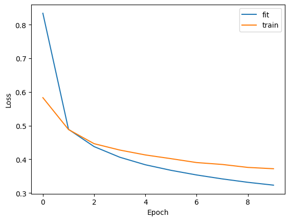
Train 0 epoch, use 7.4737 s, loss 0.8337359428405762, acc 0.7043938636779785

Test 0 epoch, use 0.9029 s, loss 0.5831130743026733, acc 0.7846449613571167

Train 1 epoch, use 6.5869 s, loss 0.4890829622745514, acc 0.8227171301841736

Test 1 epoch, use 0.1984 s, loss 0.48848050832748413, acc 0.8218347430229187

Train 2 epoch, use 6.3188 s, loss 0.43775835633277893, acc 0.8394225835800171

Test 2 epoch, use 0.2108 s, loss 0.446430504322052, acc 0.8392578363418579

Train 3 epoch, use 6.5846 s, loss 0.40623584389686584, acc 0.8518062233924866

Test 3 epoch, use 0.1735 s, loss 0.42752814292907715, acc 0.8430434465408325

Train 4 epoch, use 6.1548 s, loss 0.38380467891693115, acc 0.859663188457489

Test 4 epoch, use 0.1799 s, loss 0.41301393508911133, acc 0.8473058938980103

Train 5 epoch, use 6.2127 s, loss 0.3673246204853058, acc 0.8644005060195923

Test 5 epoch, use 0.1753 s, loss 0.4019545614719391, acc 0.8539349436759949

Train 6 epoch, use 6.1559 s, loss 0.35352981090545654, acc 0.8705119490623474

Test 6 epoch, use 0.1773 s, loss 0.3903660774230957, acc 0.8591107130050659

Train 7 epoch, use 6.1009 s, loss 0.3418504297733307, acc 0.8740192651748657

Test 7 epoch, use 0.1764 s, loss 0.38475316762924194, acc 0.860759437084198

Train 8 epoch, use 5.8664 s, loss 0.3316945731639862, acc 0.8779477477073669

Test 8 epoch, use 0.1738 s, loss 0.3759616017341614, acc 0.863493800163269

Train 9 epoch, use 5.9354 s, loss 0.323290079832077, acc 0.8812721967697144

Test 9 epoch, use 0.1778 s, loss 0.37205997109413147, acc 0.8655216097831726

import matplotlib.pyplot as plt

plt.plot(trainer.get_hist_metric('fit'), label='fit')
plt.plot(trainer.get_hist_metric('test'), label='train')
plt.xlabel("Epoch")
plt.ylabel("Loss")
plt.legend()
plt.show()

Train a SNN model

Similarly, brainpy.train.BPTT can also be used to train SNN models.

We first build a three layer SNN model:

i >> [exponential synapse] >> r >> [exponential synapse] >> o

class SNNModel(bp.DynamicalSystem):
  def __init__(self, num_in, num_rec, num_out):
    super(SNNModel, self).__init__()

    # parameters
    self.num_in = num_in
    self.num_rec = num_rec
    self.num_out = num_out

    # neuron groups
    self.r = bp.dyn.LifRef(num_rec, tau=10, V_reset=0, V_rest=0, V_th=1.)
    self.o = bp.dyn.Leaky(num_out, tau=5)

    # synapse: i->r
    self.i2r = bp.dyn.HalfProjAlignPost(comm=bp.dnn.Linear(num_in, num_rec, bp.init.KaimingNormal(scale=2.)),
                                        syn=bp.dyn.Expon(num_rec, tau=10.),
                                        out=bp.dyn.CUBA(),
                                        post=self.r)
    # synapse: r->o
    self.r2o = bp.dyn.HalfProjAlignPost(comm=bp.dnn.Linear(num_rec, num_out, bp.init.KaimingNormal(scale=2.)),
                                        syn=bp.dyn.Expon(num_out, tau=10.),
                                        out=bp.dyn.CUBA(),
                                        post=self.o)

  def update(self, spike):
    self.i2r(spike)
    self.r2o(self.r.spike.value)
    self.r()
    self.o()
    return self.o.x.value

As the model receives spiking inputs, we define functions that are necessary to transform the continuous values to spiking data.

def current2firing_time(x, tau=20., thr=0.2, tmax=1.0, epsilon=1e-7):
  x = np.clip(x, thr + epsilon, 1e9)
  T = tau * np.log(x / (x - thr))
  T = np.where(x < thr, tmax, T)
  return T

def sparse_data_generator(X, y, batch_size, nb_steps, nb_units, shuffle=True):
  labels_ = np.array(y, dtype=bm.int_)
  sample_index = np.arange(len(X))

  # compute discrete firing times
  tau_eff = 2. / bm.get_dt()
  unit_numbers = np.arange(nb_units)
  firing_times = np.array(current2firing_time(X, tau=tau_eff, tmax=nb_steps), dtype=bm.int_)

  if shuffle:
    np.random.shuffle(sample_index)

  counter = 0
  number_of_batches = len(X) // batch_size
  while counter < number_of_batches:
    batch_index = sample_index[batch_size * counter:batch_size * (counter + 1)]
    all_batch, all_times, all_units = [], [], []
    for bc, idx in enumerate(batch_index):
      c = firing_times[idx] < nb_steps
      times, units = firing_times[idx][c], unit_numbers[c]
      batch = bc * np.ones(len(times), dtype=bm.int_)
      all_batch.append(batch)
      all_times.append(times)
      all_units.append(units)
    all_batch = np.concatenate(all_batch).flatten()
    all_times = np.concatenate(all_times).flatten()
    all_units = np.concatenate(all_units).flatten()
    x_batch = bm.zeros((batch_size, nb_steps, nb_units))
    x_batch[all_batch, all_times, all_units] = 1.
    y_batch = bm.asarray(labels_[batch_index])
    yield x_batch, y_batch
    counter += 1

Now, we can define a BP trainer for this SNN model.

def loss_fun(predicts, targets):
    predicts, mon = predicts
    # L1 loss on total number of spikes
    l1_loss = 1e-5 * bm.sum(mon['r.spike'])
    # L2 loss on spikes per neuron
    l2_loss = 1e-5 * bm.mean(bm.sum(bm.sum(mon['r.spike'], axis=0), axis=0) ** 2)
    # predictions
    predicts = bm.max(predicts, axis=1)
    loss = bp.losses.cross_entropy_loss(predicts, targets)
    acc = bm.mean(predicts.argmax(-1) == targets)
    return loss + l2_loss + l1_loss, {'acc': acc}

model = SNNModel(num_in=28*28, num_rec=100, num_out=10)

trainer = bp.BPTT(
    model,
    loss_fun=loss_fun,
    loss_has_aux=True,
    optimizer=bp.optim.Adam(lr=1e-3),
    monitors={'r.spike': model.r.spike},
)

The training process is similar to that of the ANN model, instead of the data is generated by the sparse generator function we defined above.

x_train = bm.array(train_dataset.data, dtype=bm.float_) / 255
y_train = bm.array(train_dataset.targets, dtype=bm.int_)

trainer.fit(lambda: sparse_data_generator(x_train.reshape(x_train.shape[0], -1),
                                          y_train,
                                          batch_size=256,
                                          nb_steps=100,
                                          nb_units=28 * 28),
            num_epoch=5)

/tmp/ipykernel_19349/3232911099.py:8: DeprecationWarning: __array__ implementation doesn't accept a copy keyword, so passing copy=False failed. __array__ must implement 'dtype' and 'copy' keyword arguments. To learn more, see the migration guide https://numpy.org/devdocs/numpy_2_0_migration_guide.html#adapting-to-changes-in-the-copy-keyword
  labels_ = np.array(y, dtype=bm.int_)

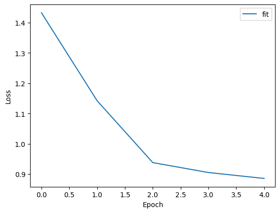
Train 0 epoch, use 46.6113 s, loss 1.4327908754348755, acc 0.4906516969203949

Train 1 epoch, use 53.4323 s, loss 1.1422044038772583, acc 0.5935329794883728

Train 2 epoch, use 52.3331 s, loss 0.9379125237464905, acc 0.6764656901359558

Train 3 epoch, use 54.1528 s, loss 0.9051787257194519, acc 0.6814736723899841

Train 4 epoch, use 52.7239 s, loss 0.8855733871459961, acc 0.6871995329856873

plt.plot(trainer.get_hist_metric('fit'), label='fit')
plt.xlabel("Epoch")
plt.ylabel("Loss")
plt.legend()
plt.show()

Customize your BP training

Actually, brainpy.train.BPTT is just one way to perform back-propagation training with your model. You can easily customize your training process.

In the below, we demonstrate how to define a BP training process by hand with the above ANN model.

# packages we need

from time import time

# define the model
model = ANNModel(28, 100, 10)

# define the loss function
def loss_fun(inputs, targets):
  runner = bp.DSTrainer(model, progress_bar=False, numpy_mon_after_run=False)
  predicts = runner.predict(inputs, reset_state=True)
  predicts = bm.max(predicts, axis=1)
  loss = bp.losses.cross_entropy_loss(predicts, targets)
  acc = bm.mean(predicts.argmax(-1) == targets)
  return loss, acc

# define the gradient function which computes the
# gradients of the trainable weights
grad_fun = bm.grad(loss_fun,
                   grad_vars=model.train_vars().unique(),
                   has_aux=True,
                   return_value=True)

# define the optimizer we need
opt = bp.optim.Adam(lr=1e-3, train_vars=model.train_vars().unique())

# training function

@bm.jit
def train(xs, ys):
  grads, loss, acc = grad_fun(xs, ys)
  opt.update(grads)
  return loss, acc

# start training

k = 0
num_batch = 256
running_loss = 0
running_acc = 0
print_step = 100
X_train = bm.asarray(x_train)
Y_train = bm.asarray(y_train)
t0 = time()
for _ in range(10):  # number of epoch
  X_train = bm.random.permutation(X_train, key=123)
  Y_train = bm.random.permutation(Y_train, key=123)

  for i in range(0, X_train.shape[0], num_batch):
    X = X_train[i: i + num_batch]
    Y = Y_train[i: i + num_batch]
    loss_, acc_ = train(X, Y)
    running_loss += loss_
    running_acc += acc_
    k += 1
    if k % print_step == 0:
      print('Step {}, Used {:.4f} s, Loss {:0.4f}, Acc {:0.4f}'.format(
        k, time() - t0,  running_loss / print_step, running_acc / print_step)
      )
      t0 = time()
      running_loss = 0
      running_acc = 0

Step 100, Used 4.0779 s, Loss 1.1585, Acc 0.6275

Step 200, Used 2.6051 s, Loss 0.5983, Acc 0.7881

Step 300, Used 3.2894 s, Loss 0.5173, Acc 0.8093

Step 400, Used 2.6218 s, Loss 0.4926, Acc 0.8180

Step 500, Used 2.6453 s, Loss 0.4678, Acc 0.8266

Step 600, Used 2.5319 s, Loss 0.4481, Acc 0.8344

Step 700, Used 2.5742 s, Loss 0.4364, Acc 0.8410

Step 800, Used 2.6635 s, Loss 0.4189, Acc 0.8453

Step 900, Used 2.5911 s, Loss 0.3937, Acc 0.8555

Step 1000, Used 2.6133 s, Loss 0.3992, Acc 0.8525

Step 1100, Used 2.5613 s, Loss 0.3838, Acc 0.8576

Step 1200, Used 2.6372 s, Loss 0.3877, Acc 0.8541

Step 1300, Used 2.6004 s, Loss 0.3724, Acc 0.8630

Step 1400, Used 2.6070 s, Loss 0.3719, Acc 0.8623

Step 1500, Used 2.6134 s, Loss 0.3565, Acc 0.8687

Step 1600, Used 2.5904 s, Loss 0.3640, Acc 0.8661

Step 1700, Used 2.6067 s, Loss 0.3492, Acc 0.8714

Step 1800, Used 2.5929 s, Loss 0.3459, Acc 0.8727

Step 1900, Used 2.6572 s, Loss 0.3416, Acc 0.8714

Step 2000, Used 2.5911 s, Loss 0.3323, Acc 0.8802

Step 2100, Used 2.5860 s, Loss 0.3393, Acc 0.8738

Step 2200, Used 2.6465 s, Loss 0.3284, Acc 0.8786

Step 2300, Used 2.5999 s, Loss 0.3273, Acc 0.8790