
braintools.surrogate.QPseudoSpike#
- class braintools.surrogate.QPseudoSpike(alpha=2.0)#
Judge spiking state with the q-PseudoSpike surrogate function [1].
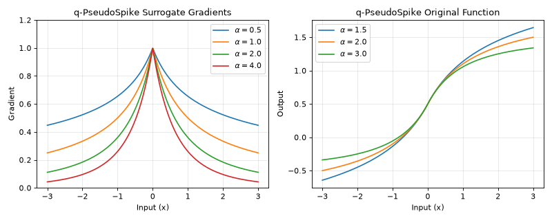
The q-PseudoSpike surrogate gradient provides a flexible framework for controlling the tail behavior of the gradient function. The parameter q (represented as alpha in the implementation) controls the tail fatness, allowing for various gradient profiles from heavy-tailed to compact support.
The forward function:
\[\begin{split}g(x) = \begin{cases} 1, & x \geq 0 \\ 0, & x < 0 \\ \end{cases}\end{split}\]The original function:
\[g_{origin}(x) = \frac{1}{2} + \mathrm{sign}(x)\, \frac{\alpha+1}{2(1-\alpha)}\left[\left(1+\frac{2|x|}{\alpha+1}\right)^{1-\alpha} - 1\right]\](the antiderivative of the backward gradient below, with a removable singularity at \(\alpha = 1\) where it equals \(0.5 + \mathrm{sign}(x)\,\frac{\alpha+1}{2}\ln(1+\frac{2|x|}{\alpha+1})\)).
Backward gradient:
\[g'(x) = (1+\frac{2|x|}{\alpha+1})^{-\alpha}\]The \(\alpha+1\) denominator (rather than \(\alpha-1\)) keeps the gradient finite for every \(\alpha > 0\), including the heavy-tailed \(\alpha < 1\) regime.
>>> import jax
>>> import jax.numpy as jnp
>>> import brainstate
>>> import braintools.surrogate as surrogate
>>> import matplotlib.pyplot as plt
>>>
>>> xs = jnp.linspace(-3, 3, 1000)
>>> fig, (ax1, ax2) = plt.subplots(1, 2, figsize=(10, 4))
>>>
>>> # Plot gradients for different alpha values
>>> for alpha in [0.5, 1.0, 2.0, 4.0]:
>>>     qps_fn = surrogate.QPseudoSpike(alpha=alpha)
>>>     grads = jax.vmap(jax.grad(qps_fn))(xs)
>>>     ax1.plot(xs, grads, label=rf'$\alpha={alpha}$')
>>>
>>> ax1.set_xlabel('Input (x)')
>>> ax1.set_ylabel('Gradient')
>>> ax1.set_title('q-PseudoSpike Surrogate Gradients')
>>> ax1.legend()
>>> ax1.grid(True, alpha=0.3)
>>> ax1.set_ylim([0, 1.2])
>>>
>>> # Plot the original (smooth) function via surrogate_fun
>>> for alpha in [1.5, 2.0, 3.0]:
>>>     qps_fn = surrogate.QPseudoSpike(alpha=alpha)
>>>     ys = jax.vmap(qps_fn.surrogate_fun)(xs)
>>>     ax2.plot(xs, ys, label=rf'$\alpha={alpha}$')
>>>
>>> ax2.set_xlabel('Input (x)')
>>> ax2.set_ylabel('Output')
>>> ax2.set_title('q-PseudoSpike Original Function')
>>> ax2.legend()
>>> ax2.grid(True, alpha=0.3)
>>> plt.tight_layout()
>>> plt.show()
(
Source code,png,hires.png,pdf)
- Parameters:
alpha (
float, optional) –Parameter to control tail fatness of gradient. Default is 2.0.
The gradient \((1 + 2|x|/(\alpha+1))^{-\alpha}\) has a power-law (polynomial) tail that is strictly positive for every finite
x; it never has compact support. Largeralphaonly makes the tail decay faster:alpha < 1: heavy, slowly decaying polynomial tail
alpha = 1:
~ 1 / (1 + |x|)polynomial tailalpha > 1: lighter polynomial tail (faster decay); still non-zero everywhere
alpha = 2:
~ |x|^-2(quadratic) decay (default)
Examples
>>> import jax
>>> import braintools.surrogate as surrogate
>>>
>>> # Create q-PseudoSpike surrogate function
>>> qps_fn = surrogate.QPseudoSpike(alpha=2.0)
>>>
>>> # Apply to input
>>> x = jax.numpy.array([-1., 0., 1.])
>>> spikes = qps_fn(x)
>>> print(spikes)
[0. 1. 1.]
>>>
>>> # Compute gradients with different tail behaviors
>>> for alpha in [0.5, 2.0, 4.0]:
...     qps_fn = surrogate.QPseudoSpike(alpha=alpha)
...     grad_fn = jax.grad(lambda x: qps_fn(x).sum())
...     grads = grad_fn(jax.numpy.array([0.5]))
...     print(f"alpha={alpha}: gradient={grads[0]:.4f}")
See also
q_pseudo_spikeFunctional version of q-PseudoSpike surrogate gradient.
SigmoidSigmoid-based surrogate gradient.
S2NNAsymmetric surrogate gradient for single-step networks.
References
Methods
__init__([alpha])surrogate_fun(x)The surrogate function.
surrogate_grad(x)The gradient function of the surrogate function.