Training with Online Algorithms

import brainpy as bp
import brainpy.math as bm
import matplotlib.pyplot as plt
import brainpy_datasets as bd

bm.set_environment(x64=True, mode=bm.batching_mode)
bm.set_platform('cpu')

bp.__version__

An NVIDIA GPU may be present on this machine, but a CUDA-enabled jaxlib is not installed. Falling back to cpu.

'2.8.0'

Online training algorithms, such as FORCE learning, have played vital roles in brain modeling. BrainPy provides brainpy.train.OnlineTrainer for model training with online algorithms.

Train a reservoir model

Here, we are going to use brainpy.OnlineTrainer to train a next generation reservoir computing model (NGRC) to predict chaotic dynamics.

We first get the training dataset.

def get_subset(data, start, end):
  res = {'x': data.xs[start: end],
         'y': data.ys[start: end],
         'z': data.zs[start: end]}
  res = bm.hstack([res['x'], res['y'], res['z']])
  # Training data must have batch size, here the batch is 1
  return res.reshape((1, ) + res.shape)

dt = 0.01
t_warmup, t_train, t_test = 5., 100., 50.  # ms
num_warmup, num_train, num_test = int(t_warmup/dt), int(t_train/dt), int(t_test/dt)

lorenz_series = bd.chaos.LorenzEq(t_warmup + t_train + t_test,
                                  dt=dt,
                                  inits={'x': 17.67715816276679,
                                         'y': 12.931379185960404,
                                         'z': 43.91404334248268})

X_warmup = get_subset(lorenz_series, 0, num_warmup - 5)
X_train = get_subset(lorenz_series, num_warmup - 5, num_warmup + num_train - 5)
X_test = get_subset(lorenz_series,
                    num_warmup + num_train - 5,
                    num_warmup + num_train + num_test - 5)

# out target data is the activity ahead of 5 time steps
Y_train = get_subset(lorenz_series, num_warmup, num_warmup + num_train)
Y_test = get_subset(lorenz_series,
                    num_warmup + num_train,
                    num_warmup + num_train + num_test)

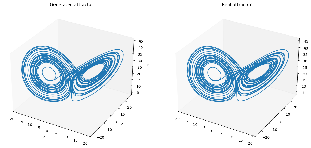
Then, we try to build a NGRC model to predict the chaotic dynamics ahead of five time steps.

class NGRC(bp.DynamicalSystemNS):
  def __init__(self, num_in):
    super(NGRC, self).__init__()
    self.r = bp.dyn.NVAR(num_in, delay=2, order=2, constant=True)
    self.o = bp.layers.Dense(self.r.num_out, num_in, b_initializer=None, mode=bm.training_mode)

  def update(self, x):
    return x >> self.r >> self.o

model = NGRC(3)
model.reset(1)

Here, we use ridge regression as the training algorithm to train the chaotic model.

trainer = bp.OnlineTrainer(model, fit_method=bp.algorithms.RLS(), dt=dt)

# first warmup the reservoir

_ = trainer.predict(X_warmup)

# then fit the reservoir model

_ = trainer.fit([X_train, Y_train])

def plot_lorenz(ground_truth, predictions):
  fig = plt.figure(figsize=(15, 10))
  ax = fig.add_subplot(121, projection='3d')
  ax.set_title("Generated attractor")
  ax.set_xlabel("$x$")
  ax.set_ylabel("$y$")
  ax.set_zlabel("$z$")
  ax.grid(False)
  ax.plot(predictions[:, 0], predictions[:, 1], predictions[:, 2])

  ax2 = fig.add_subplot(122, projection='3d')
  ax2.set_title("Real attractor")
  ax2.grid(False)
  ax2.plot(ground_truth[:, 0], ground_truth[:, 1], ground_truth[:, 2])
  plt.show()

# finally, predict the model with the test data

outputs = trainer.predict(X_test)
print('Prediction NMS: ', bp.losses.mean_squared_error(outputs, Y_test))
plot_lorenz(bm.as_numpy(Y_test).squeeze(), bm.as_numpy(outputs).squeeze())

Prediction NMS:  0.00083572382274703