Joint Differential Equations#
![]()

In a dynamical system, there may be multiple variables that change dynamically over time. Sometimes these variables are interconnected, and updating one variable requires others as the input. For example, in the widely known Hodgkin–Huxley model, the variables \(V\), \(m\), \(h\), and \(n\) are updated synchronously and interdependently (please refer to Building Neuron Modelsfor details). To achieve higher integral accuracy, it is recommended to use brainpy.JointEq to jointly solving interconnected differential equations.
import brainpy as bp
/home/chaoming/miniconda3/envs/brainx/lib/python3.13/site-packages/tqdm/auto.py:21: TqdmWarning: IProgress not found. Please update jupyter and ipywidgets. See https://ipywidgets.readthedocs.io/en/stable/user_install.html
  from .autonotebook import tqdm as notebook_tqdm
brainpy.JointEq#
brainpy.JointEq is used to merge individual but interconnected differential equations into a single joint equation. For example, below are the two differential equations of the Izhikevich model:
a, b = 0.02, 0.20
dV = lambda V, t, u, Iext: 0.04 * V * V + 5 * V + 140 - u + Iext
du = lambda u, t, V: a * (b * V - u)
Where updating \(V\) requires \(u\) as the input, and updating \(u\) requires \(V\) as the input. The joint equation can be defined as:
joint_eq = bp.JointEq(dV, du)
brainpy.JointEq receives only one argument named eqs, which can be a list or tuple containing multiple differential equations. Then it can be packed into a numarical integrator that solves the equation with a specified method, just as what can be done to any individual differential equation.
itg = bp.odeint(joint_eq, method='rk2')
There are several requirements for defining a joint equation:
Every individual differential equation should follow the format of defining a ODE or SDE funtion in BrainPy. For example, the arguments before
tdenote the dynamical variables and arguments aftertdenote the parameters.The same variable in different equations should have the same name. Different variables should named differently.
Note that brainpy.JointEq supports make nested JointEq, which means the instance of JointEq can be an element to compose a new JointEq.
Why use brainpy.JointEq?#
Users may be confused with the function of brainpy.JointEq, because multiple differential equations can be written in a single function:
def diff(V, u, t, Iext):
    dV = 0.04 * V * V + 5 * V + 140 - u + Iext
    du = a * (b * V - u)
    return dV, du

itg_V_u = bp.odeint(diff, method='rk2')
or simply packed into interators separately:
int_V = bp.odeint(dV, method='rk2')
int_u = bp.odeint(du, method='rk2')
To illusrate the difference between joint and separate differential equations, let’s dive into the differential codes of these two types of equations.
If we make numerical solver for each derivative function, they will be solved independently:
bp.odeint(dV, method='rk2', show_code=True)
def brainpy_itg_of_ode4(V, t, u, Iext, dt=0.1):
  dV_k1 = f(V, t, u, Iext)
  k2_V_arg = V + dt * dV_k1 * 0.6666666666666666
  k2_t_arg = t + dt * 0.6666666666666666
  dV_k2 = f(k2_V_arg, k2_t_arg, u, Iext)
  V_new = V + dV_k1 * dt * 0.25 + dV_k2 * dt * 0.75
  return V_new

{'f': <function <lambda> at 0x751d83a891c0>}
<brainpy.integrators.ode.explicit_rk.RK2 at 0x751c69bdcb00>
As is shown in the output code, the variable \(V\) is integrated twice by the RK2 method. For the second differential value dV_k2, the updated value of \(V\) (k2_V_arg) and original \(u\) are used to calculate the differential value. This will generate a tiny error, since the values of \(V\) and \(u\) are taken at different times.
To eliminate this error, the differential equation of \(V\) and \(u\) should be solved jointly through brainpy.JointEq:
eq = bp.JointEq(dV, du)
bp.odeint(eq, method='rk2', show_code=True)
def brainpy_itg_of_ode5_joint_eq(V, u, t, Iext, dt=0.1):
  dV_k1, du_k1 = f(V, u, t, Iext)
  k2_V_arg = V + dt * dV_k1 * 0.6666666666666666
  k2_u_arg = u + dt * du_k1 * 0.6666666666666666
  k2_t_arg = t + dt * 0.6666666666666666
  dV_k2, du_k2 = f(k2_V_arg, k2_u_arg, k2_t_arg, Iext)
  V_new = V + dV_k1 * dt * 0.25 + dV_k2 * dt * 0.75
  u_new = u + du_k1 * dt * 0.25 + du_k2 * dt * 0.75
  return V_new, u_new

{'f': <brainpy.integrators.joint_eq.JointEq object at 0x751c75b12e90>}
<brainpy.integrators.ode.explicit_rk.RK2 at 0x751cd4f24cb0>
It is shown in this output code that second differential values of \(v\) and \(u\) are calculated by using the updated values (k2_V_arg and k2_u_arg) at the same time. This will result in a more accurate integral.
Second-Order ODEs with brainpy.JointEq#
A common use case for JointEq is solving second-order ordinary differential equations (ODEs). Second-order ODEs appear in many physical systems, such as the harmonic oscillator, pendulum, or neural mass models like the Jansen-Rit model.
When using JointEq for second-order ODEs, it’s important to follow the correct function signature pattern.
Example: Harmonic Oscillator#
Consider a damped harmonic oscillator described by:
To solve this with JointEq, we split it into two first-order ODEs:
Where \(x\) is position and \(v\) is velocity.
import brainpy as bp
import brainpy.math as bm

# Parameters
k = 1.0  # spring constant
c = 0.1  # damping coefficient

# Define derivative functions
# IMPORTANT: Each state variable appears as the FIRST parameter before 't'
# Other state variables appear AFTER 't' as dependencies
def dx(x, t, v):
    """dx/dt = v"""
    return v

def dv(v, t, x):
    """dv/dt = -k*x - c*v"""
    return -k * x - c * v

# Create joint equation
joint_eq = bp.JointEq(dx, dv)
print(f"Joint equation signature: {joint_eq.__signature__}")
Joint equation signature: (x, v, t)
Important: Function Signature Pattern#
When defining derivative functions for JointEq, follow this pattern:
Correct:
def dx(x, t, v):  # x is the state variable, v is a dependency
    return v

def dv(v, t, x):  # v is the state variable, x is a dependency
    return -k * x - c * v
Incorrect:
def dx(x, v, t):  # WRONG: Both x and v before t
    return v
Rule: Each state variable should appear as the first parameter before t in exactly one derivative function. If a variable is needed as a dependency in another function, it should be placed after t.
This ensures that JointEq knows which variable each function is differentiating and which variables are dependencies.
Example: Jansen-Rit Model#
The Jansen-Rit model is a neural mass model with three coupled second-order ODEs. Here’s how to implement it correctly with JointEq:
class JansenRitModel(bp.dyn.NeuDyn):
    def __init__(self, size=1, A=3.25, te=10, B=22, ti=20, C=135,
                 e0=2.5, r=0.56, v0=6, method='rk4', **kwargs):
        super().__init__(size=size, **kwargs)
        self.A, self.te = A, te
        self.B, self.ti = B, ti
        self.C = C
        self.e0, self.r, self.v0 = e0, r, v0

        # State variables: positions (y0, y1, y2) and velocities (y3, y4, y5)
        self.y0 = bm.Variable(bm.zeros(self.num))
        self.y1 = bm.Variable(bm.zeros(self.num))
        self.y2 = bm.Variable(bm.zeros(self.num))
        self.y3 = bm.Variable(bm.zeros(self.num))  # velocity for y0
        self.y4 = bm.Variable(bm.zeros(self.num))  # velocity for y1
        self.y5 = bm.Variable(bm.zeros(self.num))  # velocity for y2

        self.integral = bp.odeint(f=self.derivative, method=method)

    # Position derivatives: dx/dt = v
    def dy0(self, y0, t, y3):  # y0 is state, y3 is dependency
        return y3 / 1000

    def dy1(self, y1, t, y4):  # y1 is state, y4 is dependency
        return y4 / 1000

    def dy2(self, y2, t, y5):  # y2 is state, y5 is dependency
        return y5 / 1000

    # Velocity derivatives: dv/dt = ...
    def dy3(self, y3, t, y0, y1, y2):  # y3 is state, others are dependencies
        Sp = 2 * self.e0 / (1 + bm.exp(self.r * (self.v0 - y1 + y2)))
        return (self.A * Sp - 2 * y3 - y0 / self.te * 1000) / self.te

    def dy4(self, y4, t, y0, y1, inp=0.):  # y4 is state, others are dependencies
        Se = 2 * self.e0 / (1 + bm.exp(self.r * (self.v0 - self.C * y0)))
        return (self.A * (inp + 0.8 * self.C * Se) - 2 * y4 - y1 / self.te * 1000) / self.te

    def dy5(self, y5, t, y0, y2):  # y5 is state, others are dependencies
        Si = 2 * self.e0 / (1 + bm.exp(self.r * (self.v0 - 0.25 * self.C * y0)))
        return (self.B * 0.25 * self.C * Si - 2 * y5 - y2 / self.ti * 1000) / self.ti

    @property
    def derivative(self):
        # Join all derivatives - order matches the state variables
        return bp.JointEq([self.dy0, self.dy1, self.dy2, self.dy3, self.dy4, self.dy5])

    def update(self, inp=0.):
        y0, y1, y2, y3, y4, y5 = self.integral(
            self.y0, self.y1, self.y2, self.y3, self.y4, self.y5,
            bp.share['t'], inp, bp.share['dt']
        )
        self.y0.value = y0
        self.y1.value = y1
        self.y2.value = y2
        self.y3.value = y3
        self.y4.value = y4
        self.y5.value = y5

# Create and test the model
model = JansenRitModel(size=1)
print("Jansen-Rit model created successfully!")
Jansen-Rit model created successfully!
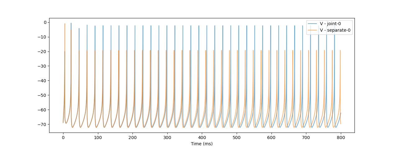
The figure below compares the simulation results of the Izhikevich model using joint and separate differential equations (\(dt = 0.2 ms\)). It is shown that as the simulation time increases, the integral error becomes greater.