brainpy.neurons.HH

class brainpy.neurons.HH(*args, input_var=True, **kwargs)

Hodgkin–Huxley neuron model.

Model Descriptions

The Hodgkin-Huxley (HH; Hodgkin & Huxley, 1952) model [1] for the generation of the nerve action potential is one of the most successful mathematical models of a complex biological process that has ever been formulated. The basic concepts expressed in the model have proved a valid approach to the study of bio-electrical activity from the most primitive single-celled organisms such as Paramecium, right through to the neurons within our own brains.

Mathematically, the model is given by,

\[ \begin{align}\begin{aligned}C \frac {dV} {dt} = -(\bar{g}_{Na} m^3 h (V &-E_{Na}) + \bar{g}_K n^4 (V-E_K) + g_{leak} (V - E_{leak})) + I(t)\\\frac {dx} {dt} &= \alpha_x (1-x) - \beta_x, \quad x\in {\rm{\{m, h, n\}}}\\&\alpha_m(V) = \frac {0.1(V+40)}{1-\exp(\frac{-(V + 40)} {10})}\\&\beta_m(V) = 4.0 \exp(\frac{-(V + 65)} {18})\\&\alpha_h(V) = 0.07 \exp(\frac{-(V+65)}{20})\\&\beta_h(V) = \frac 1 {1 + \exp(\frac{-(V + 35)} {10})}\\&\alpha_n(V) = \frac {0.01(V+55)}{1-\exp(-(V+55)/10)}\\&\beta_n(V) = 0.125 \exp(\frac{-(V + 65)} {80})\end{aligned}\end{align} \]

The illustrated example of HH neuron model please see this notebook.

The Hodgkin–Huxley model can be thought of as a differential equation system with four state variables, \(V_{m}(t),n(t),m(t)\), and \(h(t)\), that change with respect to time \(t\). The system is difficult to study because it is a nonlinear system and cannot be solved analytically. However, there are many numeric methods available to analyze the system. Certain properties and general behaviors, such as limit cycles, can be proven to exist.

1. Center manifold

Because there are four state variables, visualizing the path in phase space can be difficult. Usually two variables are chosen, voltage \(V_{m}(t)\) and the potassium gating variable \(n(t)\), allowing one to visualize the limit cycle. However, one must be careful because this is an ad-hoc method of visualizing the 4-dimensional system. This does not prove the existence of the limit cycle.

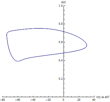
A better projection can be constructed from a careful analysis of the Jacobian of the system, evaluated at the equilibrium point. Specifically, the eigenvalues of the Jacobian are indicative of the center manifold’s existence. Likewise, the eigenvectors of the Jacobian reveal the center manifold’s orientation. The Hodgkin–Huxley model has two negative eigenvalues and two complex eigenvalues with slightly positive real parts. The eigenvectors associated with the two negative eigenvalues will reduce to zero as time \(t\) increases. The remaining two complex eigenvectors define the center manifold. In other words, the 4-dimensional system collapses onto a 2-dimensional plane. Any solution starting off the center manifold will decay towards the center manifold. Furthermore, the limit cycle is contained on the center manifold.

2. Bifurcations

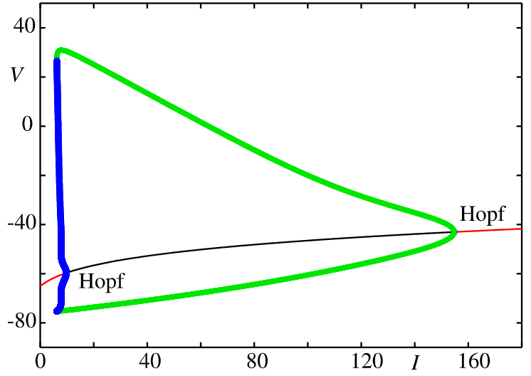
If the injected current \(I\) were used as a bifurcation parameter, then the Hodgkin–Huxley model undergoes a Hopf bifurcation. As with most neuronal models, increasing the injected current will increase the firing rate of the neuron. One consequence of the Hopf bifurcation is that there is a minimum firing rate. This means that either the neuron is not firing at all (corresponding to zero frequency), or firing at the minimum firing rate. Because of the all-or-none principle, there is no smooth increase in action potential amplitude, but rather there is a sudden “jump” in amplitude. The resulting transition is known as a canard.

The following image shows the bifurcation diagram of the Hodgkin–Huxley model as a function of the external drive \(I\) [3]. The green lines show the amplitude of a stable limit cycle and the blue lines indicate unstable limit-cycle behaviour, both born from Hopf bifurcations. The solid red line shows the stable fixed point and the black line shows the unstable fixed point.

Model Examples

>>> import brainpy as bp
>>> group = bp.neurons.HH(2)
>>> runner = bp.DSRunner(group, monitors=['V'], inputs=('input', 10.))
>>> runner.run(200.)
>>> bp.visualize.line_plot(runner.mon.ts, runner.mon.V, show=True)

>>> import brainpy as bp
>>> import brainpy.math as bm
>>> import matplotlib.pyplot as plt
>>>
>>> group = bp.neurons.HH(2)
>>>
>>> I1 = bp.inputs.spike_input(sp_times=[500., 550., 1000, 1030, 1060, 1100, 1200], sp_lens=5, sp_sizes=5., duration=2000, )
>>> I2 = bp.inputs.spike_input(sp_times=[600., 900, 950, 1500], sp_lens=5, sp_sizes=5., duration=2000, )
>>> I1 += bp.math.random.normal(0, 3, size=I1.shape)
>>> I2 += bp.math.random.normal(0, 3, size=I2.shape)
>>> I = bm.stack((I1, I2), axis=-1)
>>>
>>> runner = bp.DSRunner(group, monitors=['V'], inputs=('input', I, 'iter'))
>>> runner.run(2000.)
>>>
>>> fig, gs = bp.visualize.get_figure(1, 1, 3, 8)
>>> fig.add_subplot(gs[0, 0])
>>> plt.plot(runner.mon.ts, runner.mon.V[:, 0])
>>> plt.plot(runner.mon.ts, runner.mon.V[:, 1] + 130)
>>> plt.xlim(10, 2000)
>>> plt.xticks([])
>>> plt.yticks([])
>>> plt.show()

Parameters:

• size (sequence of int, int) – The size of the neuron group.

• ENa (float, ArrayType, Initializer, callable) – The reversal potential of sodium. Default is 50 mV.

• gNa (float, ArrayType, Initializer, callable) – The maximum conductance of sodium channel. Default is 120 msiemens.

• EK (float, ArrayType, Initializer, callable) – The reversal potential of potassium. Default is -77 mV.

• gK (float, ArrayType, Initializer, callable) – The maximum conductance of potassium channel. Default is 36 msiemens.

• EL (float, ArrayType, Initializer, callable) – The reversal potential of learky channel. Default is -54.387 mV.

• gL (float, ArrayType, Initializer, callable) – The conductance of learky channel. Default is 0.03 msiemens.

• V_th (float, ArrayType, Initializer, callable) – The threshold of the membrane spike. Default is 20 mV.

• C (float, ArrayType, Initializer, callable) – The membrane capacitance. Default is 1 ufarad.

• V_initializer (ArrayType, Initializer, callable) – The initializer of membrane potential.

• m_initializer (ArrayType, Initializer, callable) – The initializer of m channel.

• h_initializer (ArrayType, Initializer, callable) – The initializer of h channel.

• n_initializer (ArrayType, Initializer, callable) – The initializer of n channel.

• method (str) – The numerical integration method.

• name (str) – The group name.

References

[1]

Hodgkin, Alan L., and Andrew F. Huxley. “A quantitative description of membrane current and its application to conduction and excitation in nerve.” The Journal of physiology 117.4 (1952): 500.

[2]

https://en.wikipedia.org/wiki/Hodgkin%E2%80%93Huxley_model

[3]

Ashwin, Peter, Stephen Coombes, and Rachel Nicks. “Mathematical frameworks for oscillatory network dynamics in neuroscience.” The Journal of Mathematical Neuroscience 6, no. 1 (2016): 1-92.

__init__(*args, input_var=True, **kwargs)

Methods

__init__(*args[, input_var])
add_aft_update(key, fun)	Add the after update into this node
add_bef_update(key, fun)	Add the before update into this node
add_inp_fun(key, fun[, label, category])	Add an input function.
clear_input()	Empty function of clearing inputs.
cpu()	Move all variable into the CPU device.
cuda()	Move all variables into the GPU device.
dV(V, t, m, h, n, I)
dh(h, t, V)
dm(m, t, V)
dn(n, t, V)
get_aft_update(key)	Get the after update of this node by the given key.
get_batch_shape([batch_size])
get_bef_update(key)	Get the before update of this node by the given key.
get_delay_data(identifier, delay_pos, *indices)	Get delay data according to the provided delay steps.
get_delay_var(name)
get_inp_fun(key)	Get the input function.
get_local_delay(var_name, delay_name)	Get the delay at the given identifier (name).
h_alpha(V)
h_beta(V)
h_inf(V)
has_aft_update(key)	Whether this node has the after update of the given key.
has_bef_update(key)	Whether this node has the before update of the given key.
init_param(param[, shape, sharding])	Initialize parameters.
init_variable(var_data, batch_or_mode[, ...])	Initialize variables.
jit_step_run(i, *args, **kwargs)	The jitted step function for running.
load_state(state_dict, **kwargs)	Load states from a dictionary.
load_state_dict(state_dict[, warn, compatible])	Copy parameters and buffers from state_dict into this module and its descendants.
m_alpha(V)
m_beta(V)
m_inf(V)
n_alpha(V)
n_beta(V)
n_inf(V)
nodes([method, level, include_self])	Collect all children nodes.
register_delay(identifier, delay_step, ...)	Register delay variable.
register_implicit_nodes(*nodes[, node_cls])
register_implicit_vars(*variables[, var_cls])
register_local_delay(var_name, delay_name[, ...])	Register local relay at the given delay time.
reset(*args, **kwargs)	Reset function which reset the whole variables in the model (including its children models).
reset_local_delays([nodes])	Reset local delay variables.
reset_state([batch_size])
return_info()
save_state(**kwargs)	Save states as a dictionary.
setattr(key, value)	rtype: None
state_dict(**kwargs)	Returns a dictionary containing a whole state of the module.
step_run(i, *args, **kwargs)	The step run function.
sum_current_inputs(*args[, init, label])	Summarize all current inputs by the defined input functions .current_inputs.
sum_delta_inputs(*args[, init, label])	Summarize all delta inputs by the defined input functions .delta_inputs.
sum_inputs(*args, **kwargs)
to(device)	Moves all variables into the given device.
tpu()	Move all variables into the TPU device.
tracing_variable(name, init, shape[, ...])	Initialize the variable which can be traced during computations and transformations.
train_vars([method, level, include_self])	The shortcut for retrieving all trainable variables.
tree_flatten()	Flattens the object as a PyTree.
tree_unflatten(aux, dynamic_values)	Unflatten the data to construct an object of this class.
unique_name([name, type_])	Get the unique name for this object.
update([x])	The function to specify the updating rule.
update_local_delays([nodes])	Update local delay variables.
vars([method, level, include_self, ...])	Collect all variables in this node and the children nodes.

Attributes

after_updates
before_updates
cur_inputs
current_inputs
delta_inputs
derivative
implicit_nodes
implicit_vars
mode	Mode of the model, which is useful to control the multiple behaviors of the model.
name	Name of the model.
supported_modes	Supported computing modes.
varshape	The shape of variables in the neuron group.