Gradient Descent Optimizers#
![]()

Gradient descent is one of the most popular optimization methods. At present, gradient descent optimizers, combined with the loss function, are the key to machine learning, especially deep learning. In this section, we are going to understand:
how to use optimizers in BrainPy?
how to customize your own optimizer?
import brainpy as bp
import brainpy.math as bm

bp.math.set_platform('cpu')
bp.__version__
'2.4.3.post3'
import matplotlib.pyplot as plt
Optimizers in BrainPy#
The basic optimizer class in BrainPy is brainpy.optimizers.optimizer, which inludes the following optimizers:
SGD
Momentum
Nesterov momentum
Adagrad
Adadelta
RMSProp
Adam
LARS
Adan
AdamW
All supported optimizers can be inspected through the brainpy.math.optimizers APIs.
Generally, an optimizer initialization receives the learning rate lr, the trainable variables train_vars, and other hyperparameters for the specific optimizer.
lrcan be an instance of float,bm.Variableorbrainpy.optim.scheduler. However, whether it’s an instance of float orbm.Variable, it will be transformed to be an instance ofbrainpy.optim.Constantautomatically, which is a class of scheduler. Therefore, the users have to understand the type oflris actually scheduler.train_varsshould be a dict of Variable.
Here we launch a SGD optimizer.
a = bm.Variable(bm.ones((5, 4)))
b = bm.Variable(bm.zeros((3, 3)))

op = bp.optim.SGD(lr=0.001, train_vars={'a': a, 'b': b})
When you try to update the parameters, you must provide the corresponding gradients for each parameter in the update() method.
op.update({'a': bm.random.random(a.shape), 'b': bm.random.random(b.shape)})

print('a:', a)
print('b:', b)
a: Variable(value=Array([[0.9992506 , 0.9993942 , 0.99941486, 0.99976164],
                      [0.9994534 , 0.99937356, 0.9997609 , 0.999758  ],
                      [0.99927807, 0.99931985, 0.9990735 , 0.99940985],
                      [0.9995624 , 0.99956965, 0.9993627 , 0.9996619 ],
                      [0.9993749 , 0.99997044, 0.9996968 , 0.9990379 ]]),
         dtype=float32)
b: Variable(value=Array([[-0.00015692, -0.00087128, -0.00043575],
                      [-0.00018907, -0.00041636, -0.00086603],
                      [-0.00098443, -0.00046647, -0.00089446]]),
         dtype=float32)
You can process the gradients before applying them. For example, we clip the graidents by the maximum L2-norm.
grads_pre = {'a': bm.random.random(a.shape), 'b': bm.random.random(b.shape)}

grads_pre
{'a': Array(value=Array([[0.66082776, 0.4898498 , 0.3027234 , 0.52351713],
                    [0.0759604 , 0.4557693 , 0.58292365, 0.7218747 ],
                    [0.6424562 , 0.33066738, 0.39118993, 0.5811727 ],
                    [0.68779147, 0.6951357 , 0.62348413, 0.27283204],
                    [0.5947813 , 0.9510231 , 0.2681589 , 0.10165596]]),
       dtype=float32),
 'b': Array(value=Array([[0.26415503, 0.11564147, 0.08266389],
                    [0.25973928, 0.8325161 , 0.47534716],
                    [0.911289  , 0.79422164, 0.85347724]]),
       dtype=float32)}
grads_post = bm.clip_by_norm(grads_pre, 1.)

grads_post
{'a': Array(value=Array([[0.27230015, 0.20184712, 0.12473997, 0.21572004],
                    [0.03130018, 0.18780394, 0.24019904, 0.2974551 ],
                    [0.26472998, 0.13625453, 0.16119342, 0.23947756],
                    [0.2834108 , 0.28643706, 0.25691238, 0.11242295],
                    [0.24508509, 0.39187783, 0.11049735, 0.04188827]]),
       dtype=float32),
 'b': Array(value=Array([[0.14616422, 0.06398761, 0.0457402 ],
                    [0.14372088, 0.460654  , 0.26302263],
                    [0.5042412 , 0.43946463, 0.4722524 ]]),
       dtype=float32)}
op.update(grads_post)

print('a:', a)
print('b:', b)
a: Variable(value=Array([[0.9989783 , 0.99919236, 0.9992901 , 0.99954593],
                      [0.99942213, 0.99918574, 0.9995207 , 0.9994606 ],
                      [0.99901336, 0.9991836 , 0.99891233, 0.99917036],
                      [0.99927896, 0.9992832 , 0.9991058 , 0.9995495 ],
                      [0.99912983, 0.99957854, 0.9995863 , 0.998996  ]]),
         dtype=float32)
b: Variable(value=Array([[-0.00030309, -0.00093527, -0.00048149],
                      [-0.00033279, -0.00087701, -0.00112905],
                      [-0.00148868, -0.00090593, -0.00136672]]),
         dtype=float32)
Note
Optimizer usually has their own dynamically changed variables. If you JIT a function whose logic contains optimizer update, your dyn_vars in bm.jit() should include variables in Optimzier.vars().
op.vars() # SGD optimzier only has an iterable `step` variable to record the training step
{'Constant1.last_epoch': Variable(value=Array(-1), dtype=int32)}
bp.optim.Momentum(lr=0.001, train_vars={'a': a, 'b': b}).vars() # Momentum has velocity variables
{'Momentum0.a_v': Variable(value=Array([[0., 0., 0., 0.],
                       [0., 0., 0., 0.],
                       [0., 0., 0., 0.],
                       [0., 0., 0., 0.],
                       [0., 0., 0., 0.]]),
          dtype=float32),
 'Momentum0.b_v': Variable(value=Array([[0., 0., 0.],
                       [0., 0., 0.],
                       [0., 0., 0.]]),
          dtype=float32),
 'Constant2.last_epoch': Variable(value=Array(-1), dtype=int32)}
bp.optim.Adam(lr=0.001, train_vars={'a': a, 'b': b}).vars() # Adam has more variables
{'Adam1.a_m': Variable(value=Array([[0., 0., 0., 0.],
                       [0., 0., 0., 0.],
                       [0., 0., 0., 0.],
                       [0., 0., 0., 0.],
                       [0., 0., 0., 0.]]),
          dtype=float32),
 'Adam1.b_m': Variable(value=Array([[0., 0., 0.],
                       [0., 0., 0.],
                       [0., 0., 0.]]),
          dtype=float32),
 'Adam1.a_v': Variable(value=Array([[0., 0., 0., 0.],
                       [0., 0., 0., 0.],
                       [0., 0., 0., 0.],
                       [0., 0., 0., 0.],
                       [0., 0., 0., 0.]]),
          dtype=float32),
 'Adam1.b_v': Variable(value=Array([[0., 0., 0.],
                       [0., 0., 0.],
                       [0., 0., 0.]]),
          dtype=float32),
 'Constant3.last_epoch': Variable(value=Array(-1), dtype=int32)}
BrainPy also supports learning rate modification of optimizer. For example, an optimizer opt = bp.optim.Adam(lr=0.1) is created, we want to change the value lr=0.1 into lr=0.01, we can use opt.lr.lr=0.01 or opt.lr.set_value(0.01) to achieve the goal.
Here is a complete example.
import brainpy as bp
import brainpy.math as bm

dt = 0.04
num_step = int(1.0 / dt)
num_batch = 128

@bm.jit
def build_inputs_and_targets(mean=0.025, scale=0.01):
  sample = bm.random.normal(size=(num_batch, 1, 1))
  bias = mean * 2.0 * (sample - 0.5)
  samples = bm.random.normal(size=(num_batch, num_step, 1))
  noise_t = scale / dt ** 0.5 * samples
  inputs = bias + noise_t
  targets = bm.cumsum(inputs, axis=1)
  return inputs, targets

def train_data():
  for _ in range(100):
    yield build_inputs_and_targets()

class RNN(bp.DynamicalSystem):
  def __init__(self, num_in, num_hidden):
    super(RNN, self).__init__()
    self.rnn = bp.dnn.RNNCell(num_in, num_hidden, train_state=True)
    self.out = bp.dnn.Dense(num_hidden, 1)

  def update(self, x):
    return self.out(self.rnn(x))

with bm.training_environment():
    model = RNN(1, 100)

def loss(predictions, targets, l2_reg=2e-4):
    mse = bp.losses.mean_squared_error(predictions, targets)
    l2 = l2_reg * bp.losses.l2_norm(model.train_vars().unique().dict()) ** 2
    return mse + l2

opt = bp.optim.Adam(lr=0.1)
trainer = bp.BPTT(model, loss_fun=loss, optimizer=opt)
opt.lr.lr=0.01        #Modify the learning rate. You can alse use "opt.lr.set_value(0.01)"
trainer.fit(train_data, num_epoch=10)
Train 0 epoch, use 1.9907 s, loss 3.700279474258423
Train 1 epoch, use 0.7552 s, loss 0.4165635406970978
Train 2 epoch, use 0.7502 s, loss 0.07042382657527924
Train 3 epoch, use 0.7532 s, loss 0.0405302420258522
Train 4 epoch, use 0.7542 s, loss 0.027395188808441162
Train 5 epoch, use 0.7532 s, loss 0.020286478102207184
Train 6 epoch, use 0.7502 s, loss 0.01792110502719879
Train 7 epoch, use 0.7502 s, loss 0.017182694748044014
Train 8 epoch, use 0.7542 s, loss 0.016804635524749756
Train 9 epoch, use 0.7602 s, loss 0.016514629125595093
Creating A Self-Customized Optimizer#
To create your own optimization algorithm, simply inherit from bp.optim.Optimizer class and override the following methods:
__init__(): init function that receives the learning rate (lr) and trainable variables (train_vars). Do not forget to register your dynamical changed variables intoimplicit_vars.update(grads): update function that computes the updated parameters.
The general structure is shown below:
class CustomizeOp(bp.optim.Optimizer):
    def __init__(self, lr, train_vars, *params, **other_params):
        super(CustomizeOp, self).__init__(lr, train_vars)

        # customize your initialization

    def update(self, grads):
        # customize your update logic
        pass
Schedulers#
Scheduler seeks to adjust the learning rate during training through reducing the learning rate according to a pre-defined schedule. Common learning rate schedules include time-based decay, step decay and exponential decay.
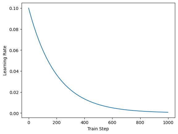
Here we set up an exponential decay scheduler, in which the learning rate will decay exponentially along the training step.
sc = bp.optim.ExponentialDecayLR(lr=0.1, decay_steps=2, decay_rate=0.99)
def show(steps, rates):
    plt.plot(steps, rates)
    plt.xlabel('Train Step')
    plt.ylabel('Learning Rate')
    plt.show()
steps = bm.arange(1000)
rates = sc(steps)

show(steps, rates)
After Optimizer initialization, the learning rate self.lr will always be an instance of bm.optimizers.Scheduler. A scalar float learning rate initialization will result in a Constant scheduler.
op.lr
Constant(lr=0.001, last_epoch=-1)
One can get the current learning rate value by calling Scheduler.__call__(i=None).
If
iis not provided, the learning rate value will be evaluated at the built-in trainingstep.Otherwise, the learning rate value will be evaluated at the given step
i.
op.lr()
0.001
In BrainPy, several commonly used learning rate schedulers are used:
Constant
StepLR
MultiStepLR
CosineAnnealingLR
ExponentialLR
ExponentialDecayLR
InverseTimeDecayLR
PolynomialDecayLR
PiecewiseConstantLR
CosineAnnealingWarmRestarts
For more details, please see the brainpy.math.optimizers APIs.
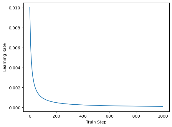
# InverseTimeDecay scheduler

rates = bp.optim.InverseTimeDecayLR(lr=0.01, decay_steps=10, decay_rate=0.999)(steps)
show(steps, rates)
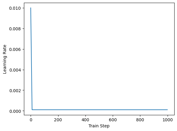
# PolynomialDecay scheduler

rates = bp.optim.PolynomialDecayLR(lr=0.01, decay_steps=10, final_lr=0.0001)(steps)
show(steps, rates)
Creating a Self-Customized Scheduler#
If users try to implement their own scheduler, simply inherit from bm.optimizers.Scheduler class and override the following methods:
__init__(): the init function.__call__(i=None): the learning rate value evalution.
class CustomizeScheduler(bp.optim.Scheduler):
    def __init__(self, lr, *params, **other_params):
        super(CustomizeScheduler, self).__init__(lr)

        # customize your initialization

    def __call__(self, i=None):
        # customize your update logic
        pass