Numerical Solvers for Fractional Differential Equations#
![]()

import matplotlib.pyplot as plt

import brainpy as bp
import brainpy.math as bm

bp.__version__
'2.4.0'
Factional differential equations have several definitions. It can be defined in a variety of different ways that do often do not all lead to the same result even for smooth functions. In neuroscience, we usually use the following two definitions:
Grünwald-Letnikov derivative
Caputo fractional derivative
See Fractional calculus - Wikipedia for more details.
Methods for Caputo FDEs#
For a given fractional differential equation
where the fractional order \(0<\alpha\le 1\). BrainPy provides two kinds of methods:
Euler method -
brainpy.fde.CaputoEulerL1 schema integration -
brainpy.fde.CaputoL1Schema
brainpy.fde.CaputoEuler#
brainpy.fed.CaputoEuler provides one-step Euler method for integrating Caputo fractional differential equations.
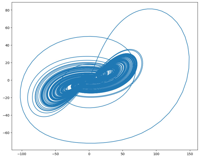
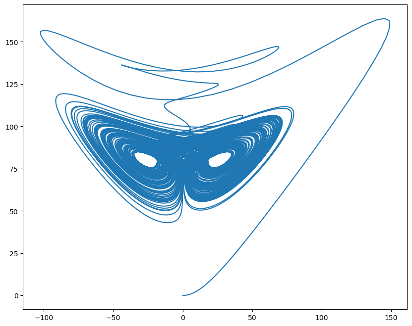
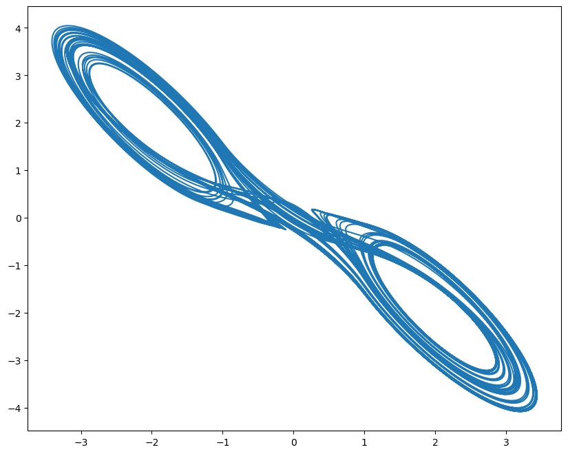
Given a fractional-order Qi chaotic system
we can solve the equation system by:
a, b, c = 35, 8 / 3, 80


def qi_system(x, y, z, t):
  dx = -a * x + a * y + y * z
  dy = c * x - y - x * z
  dz = -b * z + x * y
  return dx, dy, dz
dt = 0.001
duration = 50
inits = [0.1, 0.2, 0.3]

# The numerical integration of FDE need to know all
# history information, therefore, we need provide
# the overall simulation time "num_step" to save
# all history values.
integrator = bp.fde.CaputoEuler(qi_system,
                                alpha=0.98,  # fractional order
                                num_memory=int(duration / dt),
                                inits=inits)

runner = bp.IntegratorRunner(integrator,
                             monitors=list('xyz'),
                             inits=inits,
                             dt=dt)
runner.run(duration)
WARNING:absl:No GPU/TPU found, falling back to CPU. (Set TF_CPP_MIN_LOG_LEVEL=0 and rerun for more info.)
plt.figure(figsize=(10, 8))
plt.plot(runner.mon.x, runner.mon.y)
plt.show()
plt.figure(figsize=(10, 8))
plt.plot(runner.mon.x, runner.mon.z)
plt.show()
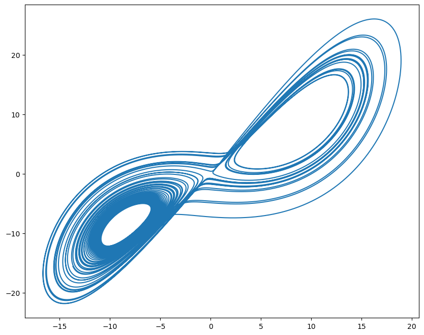
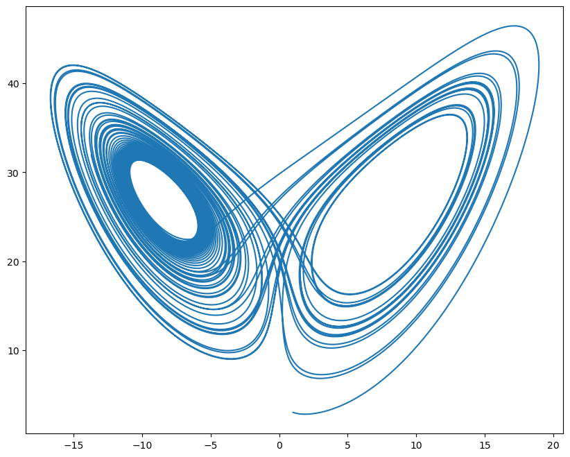
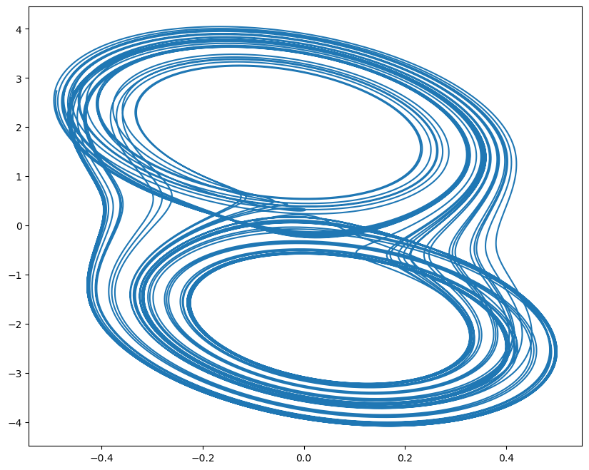
brainpy.fde.CaputoL1Schema#
brainpy.fed.CaputoL1Schema is another commonly used method to integrate Caputo derivative equations. Let’s try it with a fractional-order Lorenz system, which is given by:
a, b, c = 10, 28, 8 / 3


def lorenz_system(x, y, z, t):
  dx = a * (y - x)
  dy = x * (b - z) - y
  dz = x * y - c * z
  return dx, dy, dz
dt = 0.001
duration = 50
inits = [1, 2, 3]

integrator = bp.fde.CaputoL1Schema(lorenz_system,
                                   alpha=0.99,  # fractional order
                                   num_memory=int(duration / dt),
                                   inits=inits)

runner = bp.IntegratorRunner(integrator,
                             monitors=list('xyz'),
                             inits=inits,
                             dt=dt)
runner.run(duration)
plt.figure(figsize=(10, 8))
plt.plot(runner.mon.x, runner.mon.y)
plt.show()
plt.figure(figsize=(10, 8))
plt.plot(runner.mon.x, runner.mon.z)
plt.show()
Methods for Grünwald-Letnikov FDEs#
Grünwald-Letnikov FDE is another commonly-used type in neuroscience. Here, we provide a efficient computation method according to the short-memory principle in Grünwald-Letnikov method.
brainpy.fde.GLShortMemory#
brainpy.fde.GLShortMemory is highly efficient, because it does not require infinity memory length for numerical solution. Due to the decay property of the coefficients, brainpy.fde.GLShortMemory implements a limited memory length to reduce the computational time. Specifically, it only relies on the memory window of num_memory length. With the increasing width of memory window, the accuracy of numerical approximation will increase.
Here, we demonstrate it by using a fractional-order Chua system, which is defined as
a, b, c = 10.725, 10.593, 0.268
m0, m1 = -1.1726, -0.7872


def chua_system(x, y, z, t):
  f = m1 * x + 0.5 * (m0 - m1) * (abs(x + 1) - abs(x - 1))
  dx = a * (y - x - f)
  dy = x - y + z
  dz = -b * y - c * z
  return dx, dy, dz
dt = 0.001
duration = 200
inits = [0.2, -0.1, 0.1]

integrator = bp.fde.GLShortMemory(chua_system,
                                  alpha=[0.93, 0.99, 0.92],
                                  num_memory=1000,
                                  inits=inits)

runner = bp.IntegratorRunner(integrator,
                             monitors=list('xyz'),
                             inits=inits,
                             dt=dt)
runner.run(duration)
plt.figure(figsize=(10, 8))
plt.plot(runner.mon.x, runner.mon.z)
plt.show()
plt.figure(figsize=(10, 8))
plt.plot(runner.mon.y, runner.mon.z)
plt.show()
Actually, the coefficient used in brainpy.fde.GLWithMemory can be inspected through:
plt.figure(figsize=(10, 6))
coef = integrator.binomial_coef
alphas = bm.as_numpy(integrator.alpha)

plt.subplot(211)
for i in range(3):
  plt.plot(coef[:, i], label=r'$\alpha$=' + str(alphas[i]))
plt.legend()
plt.subplot(212)
for i in range(3):
  plt.plot(coef[:10, i], label=r'$\alpha$=' + str(alphas[i]))
plt.legend()
plt.show()
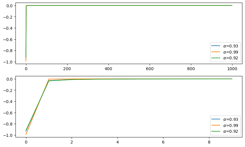
As you see, the coefficients decay very quickly!
Further reading#
More examples of how to use numerical solvers of fractional differential equations defined in BrainPy, please see: