Analyzing a Brain Dynamics Model#
![]()

In BrainPy, defined models can not only be used for simulation, but also be capable of performing automatic dynamics analysis.
BrainPy provides rich interfaces to support analysis, including
Phase plane analysis, bifurcation analysis, and fast-slow bifurcation analysis for low-dimensional systems;
linearization analysis and fixed/slow point finding for high-dimensional systems.
Here we will introduce three brief examples of 1-D bifurcation analysis and 2-D phase plane analysis. For more detailsand more examples, please refer to the tutorials of dynamics analysis.
import brainpy as bp
import brainpy.math as bm

bm.set_platform('cpu')

bm.enable_x64()  # it's better to use x64 computation
bp.__version__
'2.4.3'
Bifurcation analysis of a 1D model#
Here, we demonstrate how to perform a bifurcation analysis through a one-dimensional neuron model.
Let’s try to analyze how the external input influences the dynamics of the Exponential Integrate-and-Fire (ExpIF) model. The ExpIF model is a one-variable neuron model whose dynamics is defined by:
We can analyze the change of \({\dot {V}}\) with respect to \(V\). First, let’s generate an ExpIF model using pre-defined modules in brainpy.dyn:
expif = bp.dyn.ExpIF(1, delta_T=1.)
The default value of other parameters can be accessed directly by their names:
expif.V_rest, expif.V_T, expif.R, expif.tau
(-65.0, -59.9, 1.0, 10.0)
After defining the model, we can use it for bifurcation analysis. Note that, the following analysis
bif = bp.analysis.Bifurcation1D(
    model=expif,
    target_vars={'V': [-70., -55.]},
    target_pars={'I': [0., 6.]},
    resolutions={'I': 0.01}
)
bif.plot_bifurcation(show=True)
I am making bifurcation analysis ...
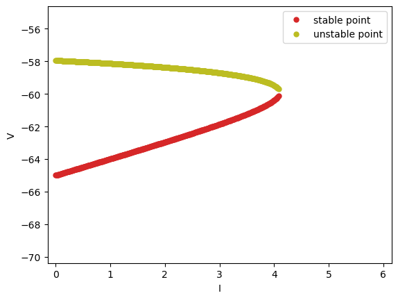
In the Bifurcation1D analyzer, model refers to the model to be analyzed (essentially the analyzer will access the derivative function in the model), target_vars denotes the target variables, target_pars denotes the changing parameters, and resolution determines the resolution of the analysis.
In the image above, there are two lines that “merge” together to form a bifurcation. The dots making up the lines refer to the fixed points of \(\mathrm{d}V/\mathrm{d}t\). On the left of the bifurcation point (where two lines merge together), there are two fixed points where \(\mathrm{d}V/\mathrm{d}t = 0\) given each external input \(I_\mathrm{ext}\). One of them is a stable point, and the other is an unstable one. When \(I_\mathrm{ext}\) increases, the two fixed points move closer to each other, overlap, and finally disappear.
Bifurcation analysis provides insights for the dynamics of the model, for it indicates the number and the change of stable states with respect to different parameters.
Phase plane analysis of a 2D model#
Besides bifurcationi analysis, another important tool is phase plane analysis, which displays the trajectory of the variable point in the vector field. Let’s take the FitzHugh–Nagumo (FHN) neuron model as an example. The dynamics of the FHN model is given by:
Users can easily define a FHN model which is also provided by BrainPy:
fhn = bp.neurons.FHN(1)
Because there are two variables, \(v\) and \(w\), in the FHN model, we shall use 2-D phase plane analysis to visualize how these two variables change over time.
analyzer = bp.analysis.PhasePlane2D(
  model=fhn,
  target_vars={'V': [-3, 3], 'w': [-3., 3.]},
  pars_update={'I_ext': 0.8},
  resolutions=0.01,
)
analyzer.plot_nullcline()
analyzer.plot_vector_field()
analyzer.plot_fixed_point()
analyzer.plot_trajectory({'V': [-2.8], 'w': [-1.8]}, duration=100.)
analyzer.show_figure()
I am computing fx-nullcline ...
I am evaluating fx-nullcline by optimization ...
I am computing fy-nullcline ...
I am evaluating fy-nullcline by optimization ...
I am creating the vector field ...
I am searching fixed points ...
I am trying to find fixed points by optimization ...
	There are 866 candidates
I am trying to filter out duplicate fixed points ...
	Found 1 fixed points.
C:\Users\adadu\miniconda3\envs\brainpy\lib\site-packages\jax\_src\numpy\array_methods.py:329: FutureWarning: The arr.split() method is deprecated. Use jax.numpy.split instead.
  warnings.warn(
	#1 V=-0.27292232484532325, w=0.5338542697682648 is a unstable node.
I am plotting the trajectory ...
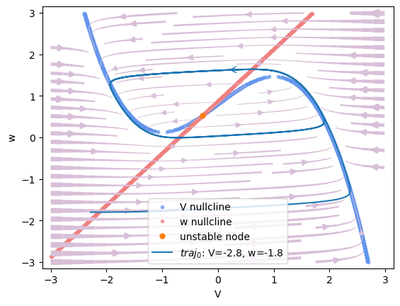
In the PhasePlane2D analyzer, the parameters model, target_vars, and resolution is the same as those in Bifurcation1D. pars_update specifies the parameters to be updated during analysis. After defining the analyzer, users can visualize the nullcline, vector field, fixed points and the trajectory in the image. The phase plane gives users intuitive interpretation of the changes of \(v\) and \(w\) guided by the vector field (violet arrows).
Slow point analysis of a high-dimensional system#
BrainPy is also capable of performing fixed/slow point analysis of high-dimensional systems. Moreover, it can perform automatic linearization analysis around the fixed point.
In the following, we use a gap junction coupled FitzHugh–Nagumo (FHN) network as an example to demonstrate how to find fixed/slow points of a high-dimensional system.
We first define the gap junction coupled FHN network as the normal DynamicalSystem class.
class GJCoupledFHN(bp.DynamicalSystem):
  def __init__(self, num=4, method='exp_auto'):
    super(GJCoupledFHN, self).__init__()

    # parameters
    self.num = num
    self.a = 0.7
    self.b = 0.8
    self.tau = 12.5
    self.gjw = 0.0001

    # variables
    self.V = bm.Variable(bm.random.uniform(-2, 2, num))
    self.w = bm.Variable(bm.random.uniform(-2, 2, num))
    self.Iext = bm.Variable(bm.zeros(num))

    # functions
    self.int_V = bp.odeint(self.dV, method=method)
    self.int_w = bp.odeint(self.dw, method=method)

  def dV(self, V, t, w, Iext=0.):
    gj = (V.reshape((-1, 1)) - V).sum(axis=0) * self.gjw
    dV = V - V * V * V / 3 - w + Iext + gj
    return dV

  def dw(self, w, t, V):
    dw = (V + self.a - self.b * w) / self.tau
    return dw

  def update(self):
    t = bp.share['t']
    dt = bp.share['dt']
    self.V.value = self.int_V(self.V, t, self.w, self.Iext, dt)
    self.w.value = self.int_w(self.w, t, self.V, dt)
    self.Iext[:] = 0.
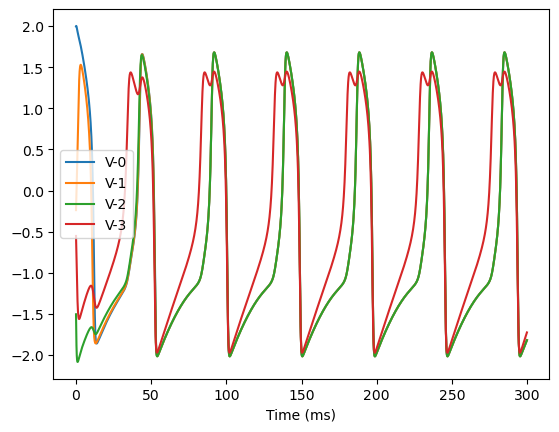
Through simulation, we can easily find that this system has a limit cycle attractor, implying that an unstable fixed point exists.
# initialize a network
model = GJCoupledFHN(4)
model.gjw = 0.1

# simulation with an input
Iext = bm.asarray([0., 0., 0., 0.6])
runner = bp.DSRunner(model, monitors=['V'], inputs=['Iext', Iext])
runner.run(300.)

# visualization
bp.visualize.line_plot(runner.mon.ts, runner.mon.V, legend='V',
                       plot_ids=list(range(model.num)),
                       show=True)
Let’s try to optimize the fixed points for this system. Note that we only take care of the variables V and w. Different from the low-dimensional analyzer, we should provide the candidate fixed points or initial fixed points when using the high-dimensional analyzer.
# init a slow point finder
finder = bp.analysis.SlowPointFinder(f_cell=model,
                                     target_vars={'V': model.V, 'w': model.w},
                                     inputs=[model.Iext, Iext])

# optimize to find fixed points
finder.find_fps_with_gd_method(
  candidates={'V': bm.random.normal(0., 2., (1000, model.num)),
              'w': bm.random.normal(0., 2., (1000, model.num))},
  tolerance=1e-6,
  num_batch=200,
  optimizer=bp.optim.Adam(lr=bp.optim.ExponentialDecay(0.05, 1, 0.9999)),
)

# filter fixed points whose loss is bigger than the threshold
finder.filter_loss(1e-8)

# remove the duplicate fixed points
finder.keep_unique()
Optimizing with Adam(lr=ExponentialDecay(0.05, decay_steps=1, decay_rate=0.9999), last_call=-1), beta1=0.9, beta2=0.999, eps=1e-08) to find fixed points:
    Batches 1-200 in 0.26 sec, Training loss 0.0002995994
    Batches 201-400 in 0.18 sec, Training loss 0.0002198732
    Batches 401-600 in 0.18 sec, Training loss 0.0001709361
    Batches 601-800 in 0.16 sec, Training loss 0.0001350801
    Batches 801-1000 in 0.19 sec, Training loss 0.0001080660
    Batches 1001-1200 in 0.19 sec, Training loss 0.0000874280
    Batches 1201-1400 in 0.18 sec, Training loss 0.0000714055
    Batches 1401-1600 in 0.18 sec, Training loss 0.0000588120
    Batches 1601-1800 in 0.17 sec, Training loss 0.0000487955
    Batches 1801-2000 in 0.20 sec, Training loss 0.0000407884
    Batches 2001-2200 in 0.19 sec, Training loss 0.0000343176
    Batches 2201-2400 in 0.19 sec, Training loss 0.0000290274
    Batches 2401-2600 in 0.16 sec, Training loss 0.0000247239
    Batches 2601-2800 in 0.18 sec, Training loss 0.0000212095
    Batches 2801-3000 in 0.16 sec, Training loss 0.0000183299
    Batches 3001-3200 in 0.18 sec, Training loss 0.0000159301
    Batches 3201-3400 in 0.16 sec, Training loss 0.0000139291
    Batches 3401-3600 in 0.17 sec, Training loss 0.0000122411
    Batches 3601-3800 in 0.18 sec, Training loss 0.0000107966
    Batches 3801-4000 in 0.17 sec, Training loss 0.0000095656
    Batches 4001-4200 in 0.17 sec, Training loss 0.0000085253
    Batches 4201-4400 in 0.17 sec, Training loss 0.0000076526
    Batches 4401-4600 in 0.16 sec, Training loss 0.0000068996
    Batches 4601-4800 in 0.17 sec, Training loss 0.0000062372
    Batches 4801-5000 in 0.18 sec, Training loss 0.0000056478
    Batches 5001-5200 in 0.17 sec, Training loss 0.0000051159
    Batches 5201-5400 in 0.16 sec, Training loss 0.0000046380
    Batches 5401-5600 in 0.17 sec, Training loss 0.0000042123
    Batches 5601-5800 in 0.18 sec, Training loss 0.0000038316
    Batches 5801-6000 in 0.18 sec, Training loss 0.0000034851
    Batches 6001-6200 in 0.17 sec, Training loss 0.0000031683
    Batches 6201-6400 in 0.18 sec, Training loss 0.0000028794
    Batches 6401-6600 in 0.19 sec, Training loss 0.0000026123
    Batches 6601-6800 in 0.18 sec, Training loss 0.0000023623
    Batches 6801-7000 in 0.17 sec, Training loss 0.0000021275
    Batches 7001-7200 in 0.16 sec, Training loss 0.0000019085
    Batches 7201-7400 in 0.19 sec, Training loss 0.0000017086
    Batches 7401-7600 in 0.17 sec, Training loss 0.0000015289
    Batches 7601-7800 in 0.20 sec, Training loss 0.0000013654
    Batches 7801-8000 in 0.18 sec, Training loss 0.0000012114
    Batches 8001-8200 in 0.18 sec, Training loss 0.0000010644
    Batches 8201-8400 in 0.17 sec, Training loss 0.0000009270
    Stop optimization as mean training loss 0.0000009270 is below tolerance 0.0000010000.
Excluding fixed points with squared speed above tolerance 1e-08:
    Kept 833/1000 fixed points with tolerance under 1e-08.
Excluding non-unique fixed points:
    Kept 1/833 unique fixed points with uniqueness tolerance 0.025.
print('fixed points:', )
finder.fixed_points
fixed points:
{'V': array([[-1.17757852, -1.17757852, -1.17757852, -0.81465053]]),
 'w': array([[-0.59697314, -0.59697314, -0.59697314, -0.14331316]])}
print('fixed point losses:', )
finder.losses
fixed point losses:
array([4.28142148e-25])
Let’s perform the linearization analysis of the found fixed points, and visualize its decomposition results.
_ = finder.compute_jacobians(finder.fixed_points, plot=True)
C:\Users\adadu\miniconda3\envs\brainpy\lib\site-packages\jax\_src\numpy\array_methods.py:329: FutureWarning: The arr.split() method is deprecated. Use jax.numpy.split instead.
  warnings.warn(
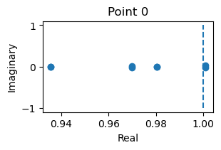
This is an unstable fixed point, because one of its eigenvalues has the real part bigger than 1.
Further reading#
For more details about how to perform bifurcation analysis and phase plane analysis, please see the tutorial of Low-dimensional Analyzers.
A good example of phase plane analysis and bifurcation analysis is the decision-making model, please see the tutorial in Analysis of a Decision-making Model
If you want to how to analyze the slow points (or fixed points) of your high-dimensional dynamical models, please see the tutorial of High-dimensional Analyzers