Introduction to Echo State Network

@Chaoming Wang

import brainpy as bp
import brainpy.math as bm

# enable x64 computation
bm.set_environment(x64=True, mode=bm.batching_mode)
bm.set_platform('cpu')

bp.__version__

'2.4.0'

import brainpy_datasets as bd
bd.__version__

'0.0.0.3'

import matplotlib.pyplot as plt

Echo State Network

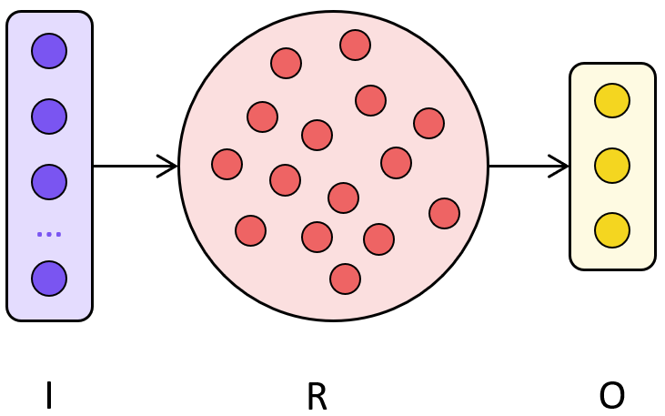
Echo State Networks (ESNs) are applied to supervised temporal machine learning tasks where for a given training input signal \(x(n)\) a desired target output signal \(y^{target}(n)\) is known. Here \(n=1, ..., T\) is the discrete time and \(T\) is the number of data points in the training dataset.

The task is to learn a model with output \(y(n)\), where \(y(n)\) matches \(y^{target}(n)\) as well as possible, minimizing an error measure \(E(y, y^{target})\), and, more importantly, generalizes well to unseen data.

ESNs use an RNN type with leaky-integrated discrete-time continuous-value units. The typical update equations are

\[\begin{split} \hat{h}(n) = \tanh(W^{in} x(n) + W^{rec}h(n-1) + W^{fb}y(n-1) + b^{rec}) \\ h(n) = (1 - \alpha) x(n-1)+\alpha \hat{h}(n) \end{split}\]

where \(h(n)\) is a vector of reservoir neuron activations, \(W^{in}\) and \(W^{rec}\) are the input and recurrent weight matrices respectively, and \(\alpha \in (0, 1]\) is the leaking rate. The model is also sometimes used without the leaky integration, which is a special case of \(\alpha=1\).

The linear readout layer is defined as

\[ y(n) = W^{out} h(n) + b^{out} \]

where \(y(n)\) is network output, \(W^{out}\) the output weight matrix, and \(b^{out}\) is the output bias.

An additional nonlinearity can be applied to \(y(n)\), as well as feedback connections \(W^{fb}\) from \(y(n-1)\) to \(\hat{h}(n)\).

A graphical representation of an ESN illustrating our notation and the idea for training is depicted in the following figure.

Ridge regression

Finding the optimal weights \(W^{out}\) that minimize the squared error between \(y(n)\) and \(y^{target}(n)\) amounts to solving a typically overdetermined system of linear equations

\[Y^{target} = W^{out}X\]

Probably the most universal and stable solution is ridge regression, also known as regression with Tikhonov regularization:

\[W^{out} = Y^{target}X^T(XX^T+\beta I)^{-1}\]

Dataset

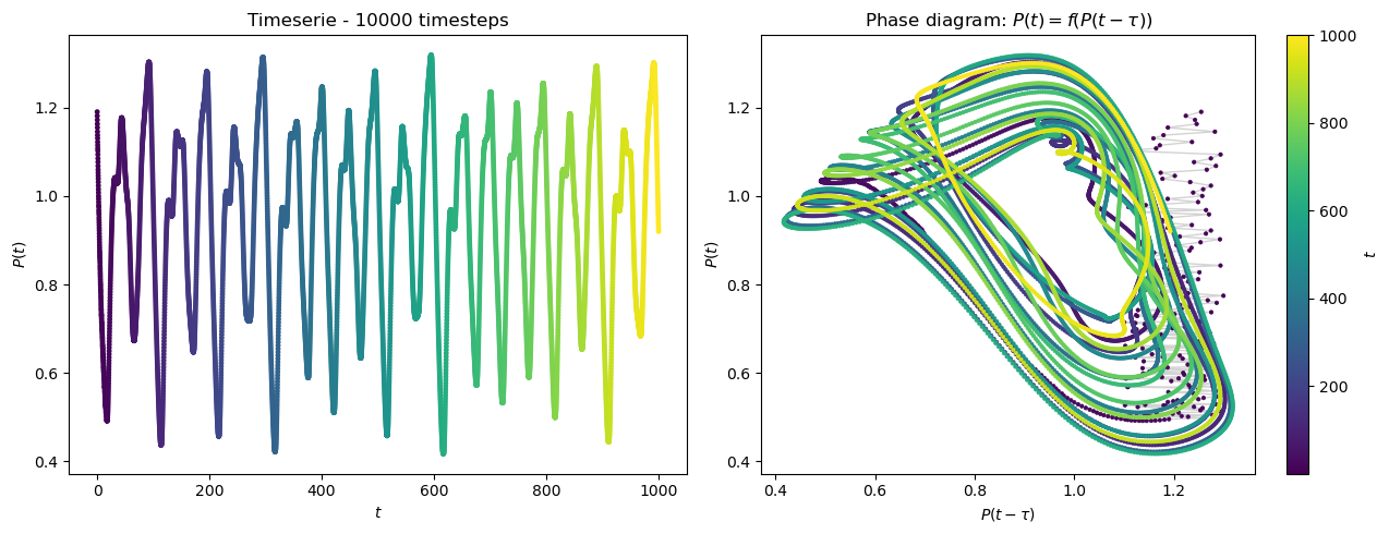
Mackey-Glass equation are a set of delayed differential equations describing the temporal behaviour of different physiological signal, for example, the relative quantity of mature blood cells over time.

The equations are defined as:

\[ \frac{dP(t)}{dt} = \frac{\beta P(t - \tau)}{1 + P(t - \tau)^n} - \gamma P(t) \]

where \(\beta = 0.2\), \(\gamma = 0.1\), \(n = 10\), and the time delay \(\tau = 17\). \(\tau\) controls the chaotic behaviour of the equations (the higher it is, the more chaotic the timeserie becomes. \(\tau=17\) already gives good chaotic results.)

def plot_mackey_glass_series(ts, x_series, x_tau_series, num_sample):
  plt.figure(figsize=(13, 5))

  plt.subplot(121)
  plt.title(f"Timeserie - {num_sample} timesteps")
  plt.plot(ts[:num_sample], x_series[:num_sample], lw=2, color="lightgrey", zorder=0)
  plt.scatter(ts[:num_sample], x_series[:num_sample], c=ts[:num_sample], cmap="viridis", s=6)
  plt.xlabel("$t$")
  plt.ylabel("$P(t)$")

  ax = plt.subplot(122)
  ax.margins(0.05)
  plt.title(f"Phase diagram: $P(t) = f(P(t-\\tau))$")
  plt.plot(x_tau_series[: num_sample], x_series[: num_sample], lw=1, color="lightgrey", zorder=0)
  plt.scatter(x_tau_series[:num_sample], x_series[: num_sample], lw=0.5, c=ts[:num_sample], cmap="viridis", s=6)
  plt.xlabel("$P(t-\\tau)$")
  plt.ylabel("$P(t)$")
  cbar = plt.colorbar()
  cbar.ax.set_ylabel('$t$')

  plt.tight_layout()
  plt.show()

An easy way to get Mackey-Glass time-series data is using brainpy.dataset.mackey_glass_series(). If you want to see the details of the implementation, please see the corresponding source code.

dt = 0.1
mg_data = bd.chaos.MackeyGlassEq(25000, dt=dt, tau=17, beta=0.2, gamma=0.1, n=10)
ts = mg_data.ts
xs = mg_data.xs
ys = mg_data.ys

plot_mackey_glass_series(ts, xs, ys, num_sample=int(1000 / dt))

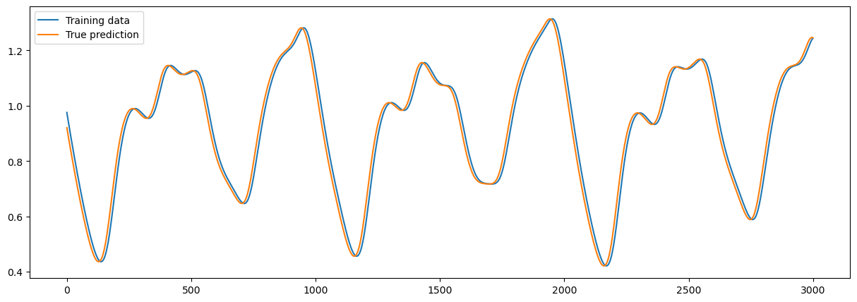
Task 1: prediction of Mackey-Glass timeseries

Predict \(P(t+1), \cdots, P(t+N)\) from \(P(t)\).

Prepare the data

def get_data(t_warm, t_forcast, t_train, sample_rate=1):
    warmup = int(t_warm / dt)  # warmup the reservoir
    forecast = int(t_forcast / dt)  # predict 10 ms ahead
    train_length = int(t_train / dt)

    X_warm = xs[:warmup:sample_rate]
    X_warm = bm.expand_dims(X_warm, 0)

    X_train = xs[warmup: warmup+train_length: sample_rate]
    X_train = bm.expand_dims(X_train, 0)

    Y_train = xs[warmup+forecast: warmup+train_length+forecast: sample_rate]
    Y_train = bm.expand_dims(Y_train, 0)

    X_test = xs[warmup + train_length: -forecast: sample_rate]
    X_test = bm.expand_dims(X_test, 0)

    Y_test = xs[warmup + train_length + forecast::sample_rate]
    Y_test = bm.expand_dims(Y_test, 0)

    return X_warm, X_train, Y_train, X_test, Y_test

# First warmup the reservoir using the first 100 ms
# Then, train the network in 20000 ms to predict 1 ms chaotic series ahead
x_warm, x_train, y_train, x_test, y_test = get_data(100, 1, 20000)

sample = 3000
fig = plt.figure(figsize=(15, 5))
plt.plot(x_train[0, :sample], label="Training data")
plt.plot(y_train[0, :sample], label="True prediction")
plt.legend()
plt.show()

Prepare the ESN

class ESN(bp.DynamicalSystemNS):
  def __init__(self, num_in, num_hidden, num_out, sr=1., leaky_rate=0.3,
               Win_initializer=bp.init.Uniform(0, 0.2)):
    super(ESN, self).__init__()
    self.r = bp.layers.Reservoir(
        num_in, num_hidden,
        Win_initializer=Win_initializer,
        spectral_radius=sr,
        leaky_rate=leaky_rate,
    )
    self.o = bp.layers.Dense(num_hidden, num_out, mode=bm.training_mode)

  def update(self, x):
    return x >> self.r >> self.o

Train and test ESN

model = ESN(1, 100, 1)
model.reset(1)
trainer = bp.RidgeTrainer(model, alpha=1e-6)

# warmup
_ = trainer.predict(x_warm)

# train
_ = trainer.fit([x_train, y_train])

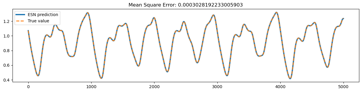
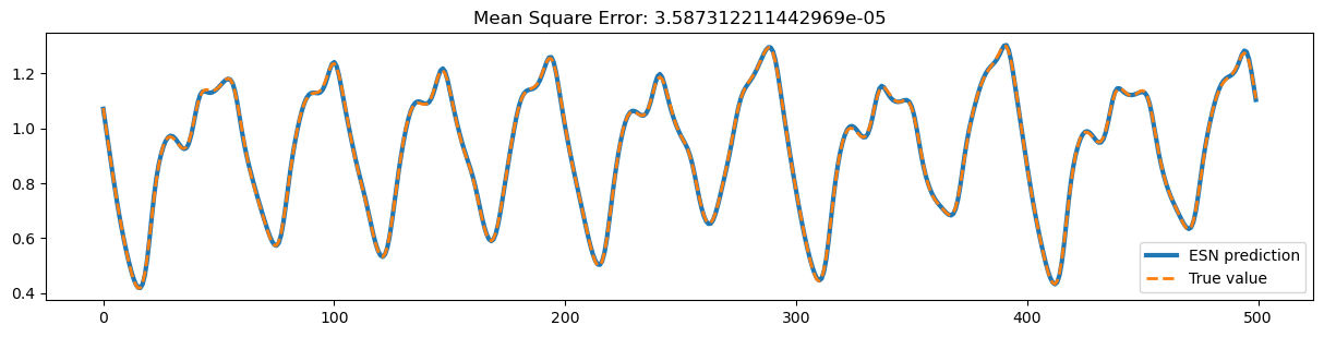
Test the training data.

ys_predict = trainer.predict(x_train)

start, end = 1000, 6000
plt.figure(figsize=(15, 7))
plt.subplot(211)
plt.plot(bm.as_numpy(ys_predict)[0, start:end, 0],
         lw=3, label="ESN prediction")
plt.plot(bm.as_numpy(y_train)[0, start:end, 0], linestyle="--",
         lw=2, label="True value")
plt.title(f'Mean Square Error: {bp.losses.mean_squared_error(ys_predict, y_train)}')
plt.legend()
plt.show()

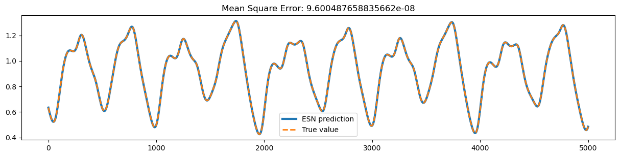
Test the testing data.

ys_predict = trainer.predict(x_test)

start, end = 1000, 6000
plt.figure(figsize=(15, 7))
plt.subplot(211)
plt.plot(bm.as_numpy(ys_predict)[0, start:end, 0], lw=3, label="ESN prediction")
plt.plot(bm.as_numpy(y_test)[0,start:end, 0], linestyle="--", lw=2, label="True value")
plt.title(f'Mean Square Error: {bp.losses.mean_squared_error(ys_predict, y_test)}')
plt.legend()
plt.show()

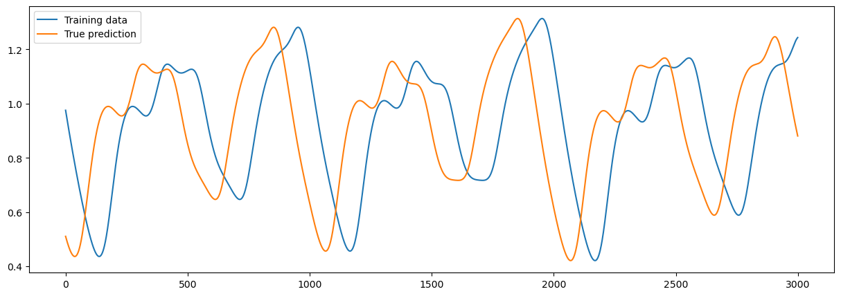
Make the task harder

# First warmup the reservoir using the first 100 ms
# Then, train the network in 20000 ms to predict 10 ms chaotic series ahead
x_warm, x_train, y_train, x_test, y_test = get_data(100, 10, 20000)

sample = 3000
plt.figure(figsize=(15, 5))
plt.plot(x_train[0, :sample], label="Training data")
plt.plot(y_train[0, :sample], label="True prediction")
plt.legend()
plt.show()

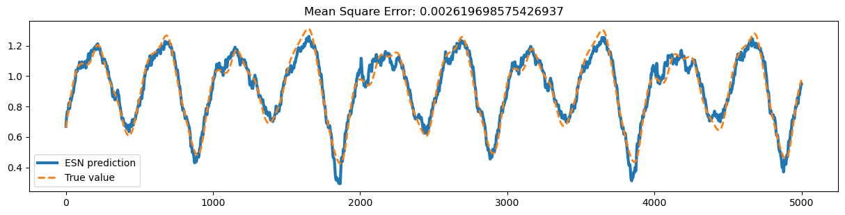
model = ESN(1, 100, 1, sr=1.1)
model.reset(1)
trainer = bp.RidgeTrainer(model, alpha=1e-6)

# warmup
_ = trainer.predict(x_warm)

# train
_ = trainer.fit([x_train, y_train])

ys_predict = trainer.predict(x_test, )

start, end = 1000, 6000
plt.figure(figsize=(15, 7))
plt.subplot(211)
plt.plot(bm.as_numpy(ys_predict)[0, start:end, 0], lw=3, label="ESN prediction")
plt.plot(bm.as_numpy(y_test)[0, start:end, 0], linestyle="--", lw=2, label="True value")
plt.title(f'Mean Square Error: {bp.losses.mean_squared_error(ys_predict, y_test)}')
plt.legend()
plt.show()

Diving into the reservoir

Let’s have a look at the effect of some of the hyperparameters of the ESN.

Spectral radius

The spectral radius is defined as the maximum eigenvalue of the reservoir matrix.

num_sample = 20
all_radius = [-0.5, 0.5, 1.25, 2.5, 10.]

plt.figure(figsize=(15, len(all_radius) * 3))
for i, s in enumerate(all_radius):
  model = ESN(1, 100, 1, sr=s)
  model.reset(1)
  runner = bp.DSTrainer(model, monitors={'state': model.r.state})
  _ = runner.predict(x_test[:, :10000])
  states = bm.as_numpy(runner.mon['state'])

  plt.subplot(len(all_radius), 1, i + 1)
  plt.plot(states[0, :, :num_sample])
  plt.ylabel(f"spectral radius=${all_radius[i]}$")
plt.xlabel(f"States ({num_sample} neurons)")
plt.show()

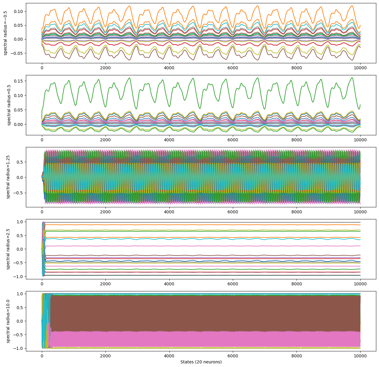
• spectral radius < 1 \(\rightarrow\) stable dynamics

• spectral radius > 1 \(\rightarrow\) chaotic dynamics

In most cases, it should have a value around \(1.0\) to ensure the echo state property (ESP): the dynamics of the reservoir should not be bound to the initial state chosen, and remains close to chaos.

This value also heavily depends on the input scaling.

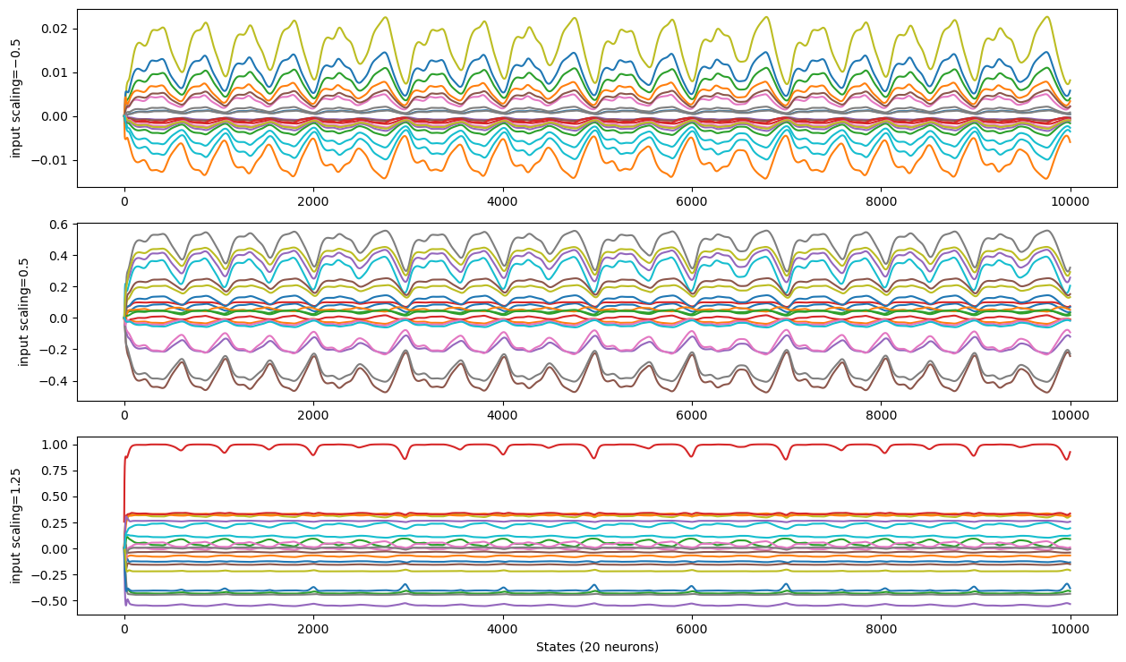
Input scaling

The input scaling controls how the ESN interact with the inputs. It is a coefficient appliyed to the input matrix \(W^{in}\).

num_sample = 20
all_input_scaling = [0.1, 1.0, 10.0]

plt.figure(figsize=(15, len(all_radius) * 3))
for i, s in enumerate(all_input_scaling):
  model = ESN(1, 100, 1, sr=1., Win_initializer=bp.init.Uniform(max_val=s))
  model.reset(1)
  runner = bp.DSTrainer(model, monitors={'state': model.r.state})
  _ = runner.predict(x_test[:, :10000])
  states = bm.as_numpy(runner.mon['state'])

  plt.subplot(len(all_radius), 1, i + 1)
  plt.plot(states[0, :, :num_sample])
  plt.ylabel(f"input scaling=${all_radius[i]}$")
plt.xlabel(f"States ({num_sample} neurons)")
plt.show()

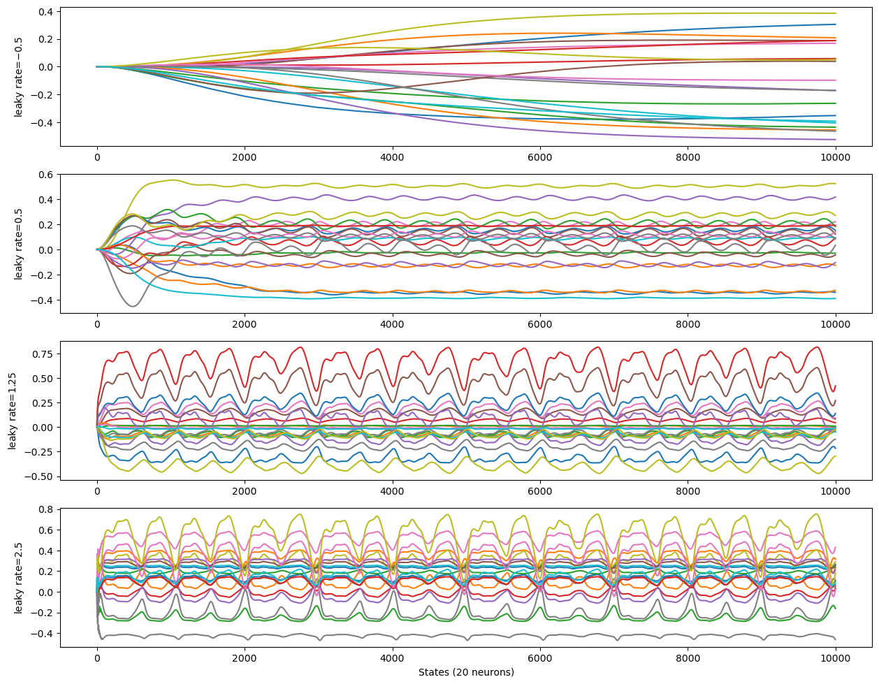
Leaking rate

The leaking rate (\(\alpha\)) controls the “memory feedback” of the ESN. The ESN states are indeed computed as:

\[ h(t+1) = \underbrace{\color{red}{(1 - \alpha)} h(t)}_{\text{previous states}} + \underbrace{\color{red}\alpha f(x(t+1), h(t))}_{\text{new states}} \]

where \(h\) is the state, \(x\) is the input data, \(f\) is the ESN model function, defined as:

\[ f(x, h) = \tanh(W^{in} \cdotp x + W^{rec} \cdotp h) \]

\(\alpha\) must be in \([0, 1]\).

num_sample = 20
all_rates = [0.001, 0.01, 0.1, 1.]

plt.figure(figsize=(15, len(all_radius) * 3))
for i, s in enumerate(all_rates):
  model = ESN(1, 100, 1, sr=1., leaky_rate=s,
              Win_initializer=bp.init.Uniform(max_val=1.), )
  model.reset(1)
  runner = bp.DSTrainer(model, monitors={'state': model.r.state})
  _ = runner.predict(x_test[:, :10000])
  states = bm.as_numpy(runner.mon['state'])

  plt.subplot(len(all_radius), 1, i + 1)
  plt.plot(states[0, :, :num_sample])
  plt.ylabel(f"leaky rate=${all_radius[i]}$")
plt.xlabel(f"States ({num_sample} neurons)")
plt.show()

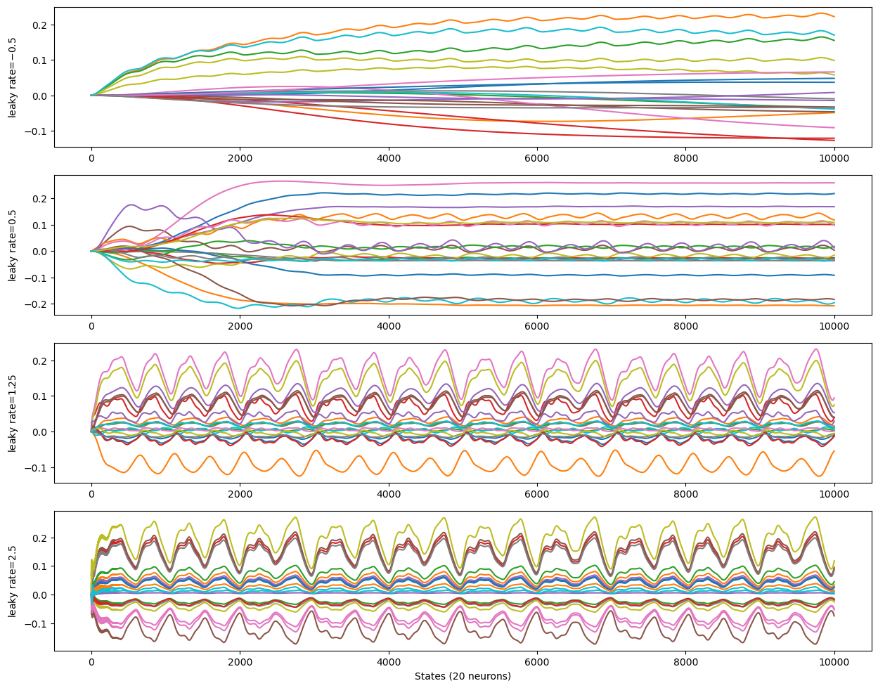
Let’s reduce the input influence to see what is happening inside the reservoir (input scaling set to 0.2):

num_sample = 20
all_rates = [0.001, 0.01, 0.1, 1.]

plt.figure(figsize=(15, len(all_radius) * 3))
for i, s in enumerate(all_rates):
  model = ESN(1, 100, 1, sr=1., leaky_rate=s,
              Win_initializer=bp.init.Uniform(max_val=.2), )
  model.reset(1)
  runner = bp.DSTrainer(model, monitors={'state': model.r.state})
  _ = runner.predict(x_test[:, :10000])
  states = bm.as_numpy(runner.mon['state'])

  plt.subplot(len(all_radius), 1, i + 1)
  plt.plot(states[0, :, :num_sample])
  plt.ylabel(f"leaky rate=${all_radius[i]}$")
plt.xlabel(f"States ({num_sample} neurons)")
plt.show()

• high leaking rate \(\rightarrow\) low inertia, little memory of previous states

• low leaking rate \(\rightarrow\) high inertia, big memory of previous states

The leaking rate can be seen as the inverse of the reservoir’s time contant.

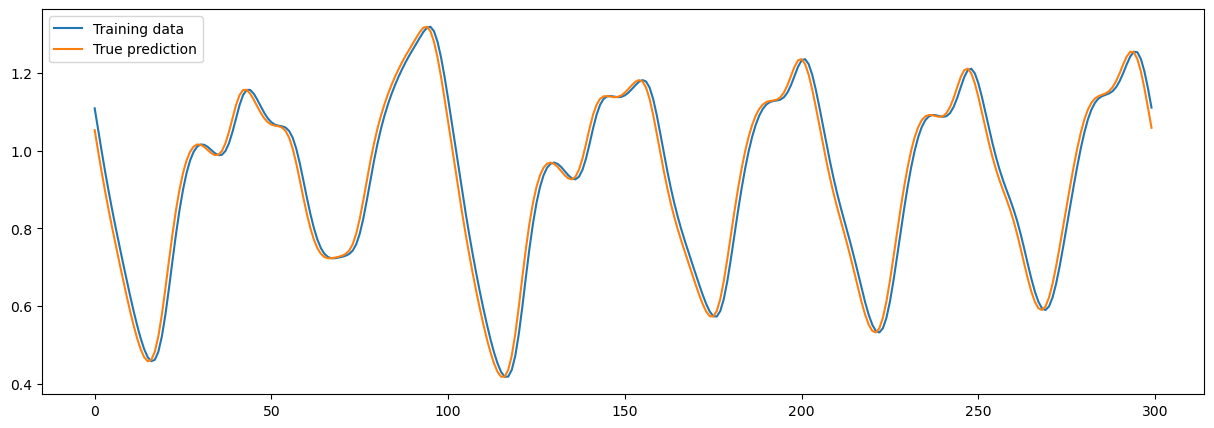
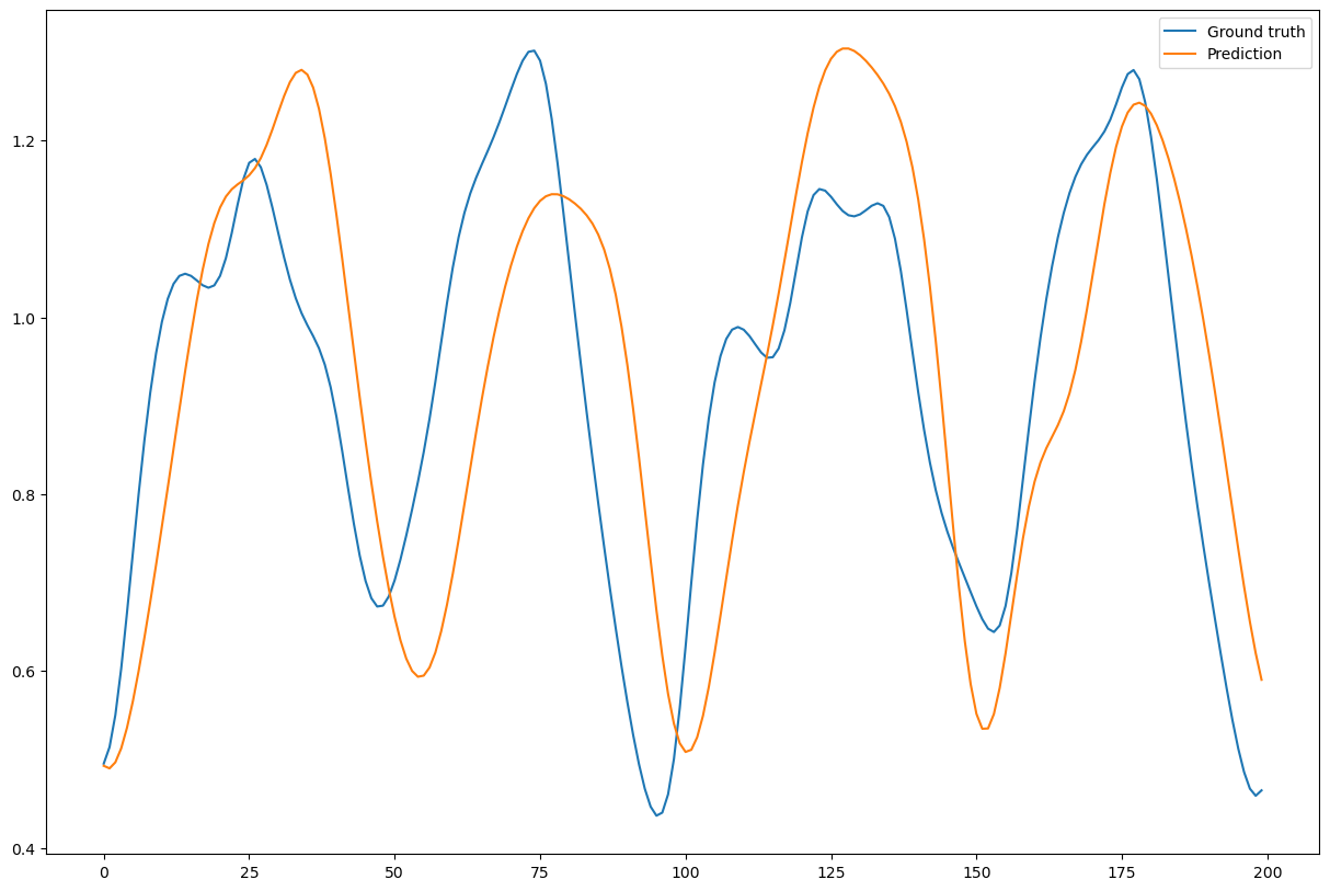
Task 2: generation of Mackey-Glass timeseries

Generative mode: the output of ESN will be used as the input.

During this task, the ESN is trained to make a short forecast of the timeserie (1 timestep ahead). Then, it will be asked to run on its own outputs, trying to predict its own behaviour.

# First warmup the reservoir using the first 500 ms
# Then, train the network in 20000 ms to predict 1 ms chaotic series ahead
x_warm, x_train, y_train, x_test, y_test = get_data(500, 1, 20000, sample_rate=int(1/dt))

sample = 300
fig = plt.figure(figsize=(15, 5))
plt.plot(x_train[0, :sample], label="Training data")
plt.plot(y_train[0, :sample], label="True prediction")
plt.legend()
plt.show()

model = ESN(1, 100, 1, sr=1.1, Win_initializer=bp.init.Uniform(max_val=.2), )
model.reset(1)
trainer = bp.RidgeTrainer(model, alpha=1e-7)

# warmup
_ = trainer.predict(x_warm)

# train
trainer.fit([x_train, y_train])

# test
ys_predict = trainer.predict(x_train)

start, end = 100, 600
plt.figure(figsize=(15, 7))
plt.subplot(211)
plt.plot(bm.as_numpy(ys_predict)[0, start:end, 0],
         lw=3, label="ESN prediction")
plt.plot(bm.as_numpy(y_train)[0, start:end, 0], linestyle="--",
         lw=2, label="True value")
plt.title(f'Mean Square Error: {bp.losses.mean_squared_error(ys_predict, y_train)}')
plt.legend()
plt.show()

jit_model = bm.jit(model)

outputs = [x_test[:, 0]]
truths = [x_test[:, 1]]
for i in range(200):
    outputs.append(jit_model(dict(), outputs[-1]))
    truths.append(x_test[:, i+2])
outputs = bm.asarray(outputs)
truths = bm.asarray(truths)

plt.figure(figsize=(15, 10))
plt.plot(bm.as_numpy(truths).squeeze()[:200], label='Ground truth')
plt.plot(bm.as_numpy(outputs).squeeze()[:200], label='Prediction')
plt.legend()
plt.show()

References

• Jaeger, H.: The “echo state” approach to analysing and training recurrent neural networks. Technical Report GMD Report 148, German National Research Center for Information Technology (2001)

• Lukoševičius, Mantas. “A Practical Guide to Applying Echo State Networks.” Neural Networks: Tricks of the Trade (2012).