Analysis of a Decision-making Model#
![]()

In this section, we are going to use the low-dimensional analyzers to make phase plane and bifurcation analysis for the decision-making model proposed by (Wong & Wang) [1].
Decision making model#
This model considers two excitatory neural assemblies, populations 1 and 2 , that compete with each other through a shared pool of inhibitory neurons. In our analysis, we use the following model equations.
Let \(r_1\) and \(r_2\) be firing rates of E and I populations, and the total synaptic input current \(I_i\) and the resulting firing rate \(r_i\) of the neural population \(i\) obey the following input-output relationship (\(F - I\) curve):
which captures the current-frequency function of a leaky integrate-and-fire neuron. The parameter values are \(a\) = 270 Hz/nA, \(b\) = 108 Hz, \(d\) = 0.154 sec.
Assume that the synaptic drive variables’ \(S_1\) and \(S_2\) obey
where \(\gamma\) = 0.641. The net current into each population is given by
The synaptic time constant is \(\tau_s\) = 100 ms (NMDA time consant). The synaptic coupling strengths are \(J_E\) = 0.2609 nA, \(J_I\) = -0.0497 nA, and \(J_{ext}\) = 0.00052 nA. Stimulus-selective inputs to populations 1 and 2 are governed by unitless parameters \(\mu_1\) and \(\mu_2\), respectively.
For the decision-making paradigm, the input rates \(\mu_1\) and \(\mu_2\) are determined by the stimulus coherence \(c'\) which ranges between 0 (0%) and 1 (100%):
import brainpy as bp
import brainpy.math as bm

bm.enable_x64()
bm.set_platform('cpu')
bp.__version__
'2.4.0'
Parameters#
gamma = 0.641  # Saturation factor for gating variable
tau = 0.1  # Synaptic time constant [sec]
a = 270.  #  Hz/nA
b = 108.  # Hz
d = 0.154  # sec

I0 = 0.3255  # background current [nA]
JE = 0.2609  # self-coupling strength [nA]
JI = -0.0497  # cross-coupling strength [nA]
JAext = 0.00052  # Stimulus input strength [nA]
Ib = 0.3255  # The background input
Model implementation#
@bp.odeint
def int_s1(s1, t, s2, coh=0.5, mu=20.):
    I1 = JE * s1 + JI * s2 + Ib + JAext * mu * (1. + coh)
    r1 = (a * I1 - b) / (1. - bm.exp(-d * (a * I1 - b)))
    return - s1 / tau + (1. - s1) * gamma * r1

@bp.odeint
def int_s2(s2, t, s1, coh=0.5, mu=20.):
    I2 = JE * s2 + JI * s1 + Ib + JAext * mu * (1. - coh)
    r2 = (a * I2 - b) / (1. - bm.exp(-d * (a * I2 - b)))
    return - s2 / tau + (1. - s2) * gamma * r2
Phase plane analysis#
The advantage of the reduced model is that we can understand what dynamical behaviors the model generate for a particular parmeter set using phase-plane analysis and the explore how this behavior changed when the model parameters are varied (bifurcation analysis).
To this end, we will use brainpy.analysis module.
We construct the phase portraits of the reduced model for different stimulus inputs (see Figure 4 and Figure 5 in (Wong & Wang, 2006) [1]).
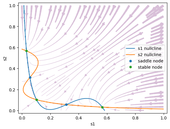
No stimulus: \(\mu_0 =0\) Hz. In the absence of a stimulus, the two nullclines intersect with each other five times, producing five steady states, of which three are stable (attractors) and two are unstable
analyzer = bp.analysis.PhasePlane2D(
    model=[int_s1, int_s2],
    target_vars={'s1': [0, 1], 's2': [0, 1]},
    pars_update={'mu': 0.},
    resolutions=0.001,
)
analyzer.plot_vector_field()
analyzer.plot_nullcline(coords=dict(s2='s2-s1'),
                        x_style={'fmt': '-'},
                        y_style={'fmt': '-'})
analyzer.plot_fixed_point()
analyzer.show_figure()
I am creating the vector field ...
I am computing fx-nullcline ...
I am evaluating fx-nullcline by optimization ...
I am computing fy-nullcline ...
I am evaluating fy-nullcline by optimization ...
I am searching fixed points ...
I am trying to find fixed points by optimization ...
	There are 1212 candidates
I am trying to filter out duplicate fixed points ...
	Found 5 fixed points.
	#1 s1=0.5669871605297269, s2=0.031891419715715866 is a stable node.
	#2 s1=0.31384492489135923, s2=0.055785333471845625 is a saddle node.
	#3 s1=0.1026514458219984, s2=0.10265095098914433 is a stable node.
	#4 s1=0.05578534267632889, s2=0.3138449310808786 is a saddle node.
	#5 s1=0.03189144636489119, s2=0.5669870352865433 is a stable node.
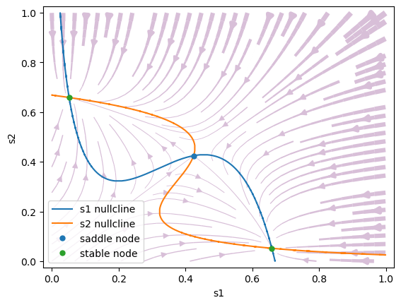
Symmetric stimulus: \(\mu_0=30\) Hz, \(c'=0\). When a stimulus is applied, the phase space of the model is reconfigured. The spontaneous state vanishes. At the same time, a saddle-type unstable steady state is created that separates the two asymmetrical attractors.
analyzer = bp.analysis.PhasePlane2D(
    model=[int_s1, int_s2],
    target_vars={'s1': [0, 1], 's2': [0, 1]},
    pars_update={'mu': 30., 'coh': 0.},
    resolutions=0.001,
)
analyzer.plot_vector_field()
analyzer.plot_nullcline(coords=dict(s2='s2-s1'),
                        x_style={'fmt': '-'},
                        y_style={'fmt': '-'})
analyzer.plot_fixed_point()
analyzer.show_figure()
I am creating the vector field ...
I am computing fx-nullcline ...
I am evaluating fx-nullcline by optimization ...
I am computing fy-nullcline ...
I am evaluating fy-nullcline by optimization ...
I am searching fixed points ...
I am trying to find fixed points by optimization ...
	There are 1212 candidates
I am trying to filter out duplicate fixed points ...
	Found 3 fixed points.
	#1 s1=0.658694232143127, s2=0.05180719943991283 is a stable node.
	#2 s1=0.4244557898485833, s2=0.4244556283731397 is a saddle node.
	#3 s1=0.05180717720080605, s2=0.6586942355713474 is a stable node.
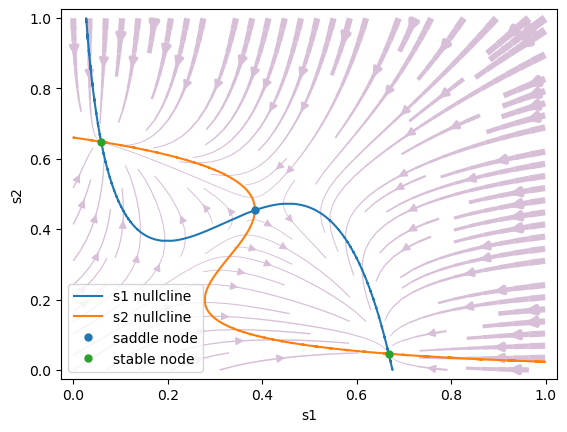
Biased stimulus: \(\mu_0=30\) Hz, \(c' = 0.14\) (14 % coherence). The phase space changes when a weak motion stimulus is presented. The phase space is no longer symmetrical: the attractor state s1 (correct choice) has a larger basin of attraction than attractor s2.
analyzer = bp.analysis.PhasePlane2D(
    model=[int_s1, int_s2],
    target_vars={'s1': [0, 1], 's2': [0, 1]},
    pars_update={'mu': 30., 'coh': 0.14},
    resolutions=0.001,
)
analyzer.plot_vector_field()
analyzer.plot_nullcline(coords=dict(s2='s2-s1'),
                        x_style={'fmt': '-'},
                        y_style={'fmt': '-'})
analyzer.plot_fixed_point()
analyzer.show_figure()
I am creating the vector field ...
I am computing fx-nullcline ...
I am evaluating fx-nullcline by optimization ...
I am computing fy-nullcline ...
I am evaluating fy-nullcline by optimization ...
I am searching fixed points ...
I am trying to find fixed points by optimization ...
	There are 1212 candidates
I am trying to filter out duplicate fixed points ...
	Found 3 fixed points.
	#1 s1=0.6679776124172938, s2=0.04583022226100692 is a stable node.
	#2 s1=0.38455860789855495, s2=0.4536309035289815 is a saddle node.
	#3 s1=0.059110032802350894, s2=0.6481046659437735 is a stable node.
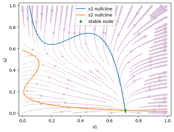
Stimulus to one population only: \(\mu_0=30\) Hz, \(c'=1.\) (100 % coherence). When \(c'\) is sufficiently large, the saddle steady state annihilates with the less favored attractor, leaving only one choice attractor.
analyzer = bp.analysis.PhasePlane2D(
    model=[int_s1, int_s2],
    target_vars={'s1': [0, 1], 's2': [0, 1]},
    pars_update={'mu': 30., 'coh': 1.},
    resolutions=0.001,
)
analyzer.plot_vector_field()
analyzer.plot_nullcline(coords=dict(s2='s2-s1'),
                        x_style={'fmt': '-'},
                        y_style={'fmt': '-'})
analyzer.plot_fixed_point()
analyzer.show_figure()
I am creating the vector field ...
I am computing fx-nullcline ...
I am evaluating fx-nullcline by optimization ...
I am computing fy-nullcline ...
I am evaluating fy-nullcline by optimization ...
I am searching fixed points ...
I am trying to find fixed points by optimization ...
	There are 1212 candidates
I am trying to filter out duplicate fixed points ...
	Found 1 fixed points.
	#1 s1=0.7092805209334904, s2=0.023963663041994612 is a stable node.
Bifurcation analysis#
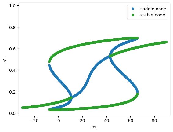
To see how the phase portrait of the system changed when we chang the stimulus current, we will generate a bifurcation diagram for the reduced model. On the bifurcation diagram the fixed points of the model are shown as a function of a changing parameter.
In the next, we generate bifurcation diagrams with the different parameters.
Fix the coherence \(c'=0\), vary the stimulus strength \(\mu_0\). See Figure 10 in (Wong & Wang, 2006) [1].
analyzer = bp.analysis.Bifurcation2D(
  model=[int_s1, int_s2],
  target_vars={'s1': [0., 1.], 's2': [0., 1.]},
  target_pars={'mu': [-30., 90.]},
  pars_update={'coh': 0.},
  resolutions={'mu': 0.2},
)
analyzer.plot_bifurcation(num_rank=50)
analyzer.show_figure()
I am making bifurcation analysis ...
I am filtering out fixed point candidates with auxiliary function ...
I am trying to find fixed points by optimization ...
	There are 30000 candidates
I am trying to filter out duplicate fixed points ...
	Found 1744 fixed points.

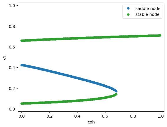
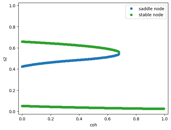
Fix the stimulus strength \(\mu_0 = 30\) Hz, vary the coherence \(c'\).
analyzer = bp.analysis.Bifurcation2D(
  model=[int_s1, int_s2],
  target_vars={'s1': [0., 1.], 's2': [0., 1.]},
  target_pars={'coh': [0., 1.]},
  pars_update={'mu': 30.},
  resolutions={'coh': 0.005},
)
analyzer.plot_bifurcation(num_rank=50)
analyzer.show_figure()
I am making bifurcation analysis ...
I am filtering out fixed point candidates with auxiliary function ...
I am trying to find fixed points by optimization ...
	There are 10000 candidates
I am trying to filter out duplicate fixed points ...
	Found 474 fixed points.
References#
[1] Wong K-F and Wang X-J (2006). A recurrent network mechanism for time integration in perceptual decisions. J. Neurosci 26, 1314-1328.