MidPoint#
- class brainpy.integrators.ode.MidPoint(f, var_type=None, dt=None, name=None, show_code=False, state_delays=None, neutral_delays=None)[source]#
Explicit midpoint method for ODEs.
Also known as the modified Euler method [1].
The midpoint method is a one-step method for numerically solving the differential equation given by:
\[y'(t) = f(t, y(t)), \quad y(t_0) = y_0 .\]The formula of the explicit midpoint method is:
\[y_{n+1} = y_n + hf\left(t_n+\frac{h}{2},y_n+\frac{h}{2}f(t_n, y_n)\right).\]Therefore, the Butcher tableau of the midpoint method is:
\[\begin{split}\begin{array}{c|cc} 0 & 0 & 0 \\ 1 / 2 & 1 / 2 & 0 \\ \hline & 0 & 1 \end{array}\end{split}\]Derivation
Compared to the slope formula of Euler method \(y'(t) \approx \frac{y(t+h) - y(t)}{h}\), the midpoint method use
\[y'\left(t+\frac{h}{2}\right) \approx \frac{y(t+h) - y(t)}{h},\]The reason why we use this, please see the following geometric interpretation. Then, we get
\[y(t+h) \approx y(t) + hf\left(t+\frac{h}{2},y\left(t+\frac{h}{2}\right)\right).\]However, we do not know \(y(t+h/2)\). The solution is then to use a Taylor series expansion exactly as the Euler method to solve:
\[y\left(t + \frac{h}{2}\right) \approx y(t) + \frac{h}{2}y'(t)=y(t) + \frac{h}{2}f(t, y(t)),\]Finally, we can get the final step function:
\[y(t + h) \approx y(t) + hf\left(t + \frac{h}{2}, y(t) + \frac{h}{2}f(t, y(t))\right).\]Geometric interpretation
In the basic Euler’s method, the tangent of the curve at \((t_{n},y_{n})\) is computed using \(f(t_{n},y_{n})\). The next value \(y_{n+1}\) is found where the tangent intersects the vertical line \(t=t_{n+1}\). However, if the second derivative is only positive between \(t_{n}\) and \(t_{n+1}\), or only negative, the curve will increasingly veer away from the tangent, leading to larger errors as \(h\) increases.
Compared with the Euler method, midpoint method use the tangent at the midpoint (upper, green line segment in the following figure [2]), which would most likely give a more accurate approximation of the curve in that interval.
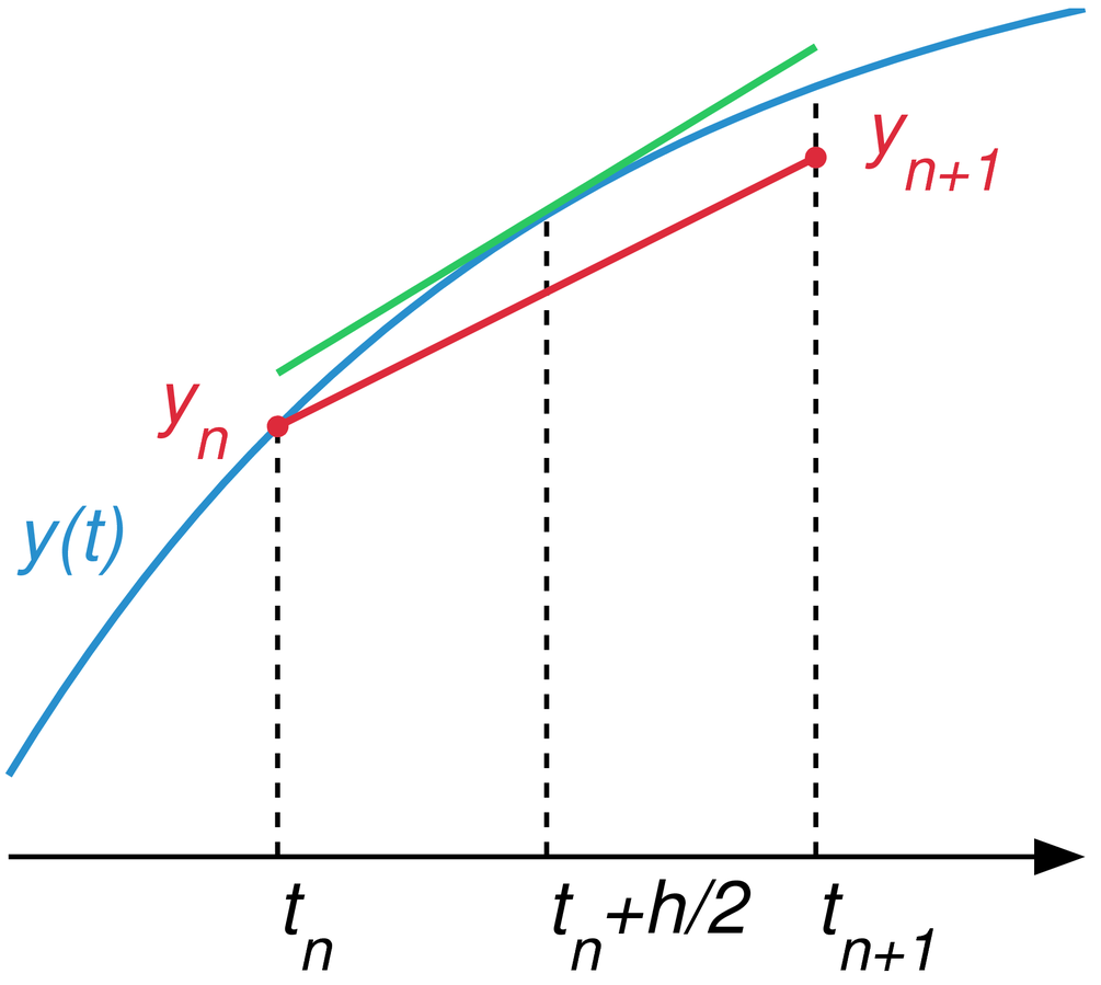
Although this midpoint tangent could not be accurately calculated, we can estimate midpoint value of \(y(t)\) by using the original Euler’s method. Finally, the improved tangent is used to calculate the value of \(y_{n+1}\) from \(y_{n}\). This last step is represented by the red chord in the diagram.
Note
Note that the red chord is not exactly parallel to the green segment (the true tangent), due to the error in estimating the value of \(y(t)\) at the midpoint.
References