Training with Offline Algorithms

import brainpy as bp
import brainpy.math as bm
import brainpy_datasets as bd
import matplotlib.pyplot as plt

bm.set_environment(x64=True, mode=bm.batching_mode)
bm.set_platform('cpu')

bp.__version__

'2.4.0'

BrainPy provides many offline training algorithms can help users train models such as reservoir computing models.

Train a reservoir model

Here, we train an echo-state machine to predict chaotic dynamics. This example is used to illustrate how to use brainpy.train.OfflineTrainer.

We first get the training dataset.

def get_subset(data, start, end):
  res = {'x': data.xs[start: end],
         'y': data.ys[start: end],
         'z': data.zs[start: end]}
  res = bm.hstack([res['x'], res['y'], res['z']])
  # Training data must have batch size, here the batch is 1
  return res.reshape((1, ) + res.shape)

dt = 0.01
t_warmup, t_train, t_test = 5., 100., 50.  # ms
num_warmup, num_train, num_test = int(t_warmup/dt), int(t_train/dt), int(t_test/dt)

lorenz_series = bd.chaos.LorenzEq(t_warmup + t_train + t_test,
                                  dt=dt,
                                  inits={'x': 17.67715816276679,
                                         'y': 12.931379185960404,
                                         'z': 43.91404334248268})

X_warmup = get_subset(lorenz_series, 0, num_warmup - 5)
X_train = get_subset(lorenz_series, num_warmup - 5, num_warmup + num_train - 5)
X_test = get_subset(lorenz_series,
                    num_warmup + num_train - 5,
                    num_warmup + num_train + num_test - 5)

# out target data is the activity ahead of 5 time steps
Y_train = get_subset(lorenz_series, num_warmup, num_warmup + num_train)
Y_test = get_subset(lorenz_series,
                    num_warmup + num_train,
                    num_warmup + num_train + num_test)

Then, we try to build an echo-state machine to predict the chaotic dynamics ahead of five time steps.

class ESN(bp.DynamicalSystemNS):
  def __init__(self, num_in, num_hidden, num_out):
    super(ESN, self).__init__()
    self.r = bp.layers.Reservoir(num_in, num_hidden,
                                 Win_initializer=bp.init.Uniform(-0.1, 0.1),
                                 Wrec_initializer=bp.init.Normal(scale=0.1),
                                 in_connectivity=0.02,
                                 rec_connectivity=0.02,
                                 comp_type='dense')
    self.o = bp.layers.Dense(num_hidden, num_out, W_initializer=bp.init.Normal(),
                             mode=bm.training_mode)

  def update(self, x):
    return x >> self.r >> self.o

model = ESN(3, 100, 3)

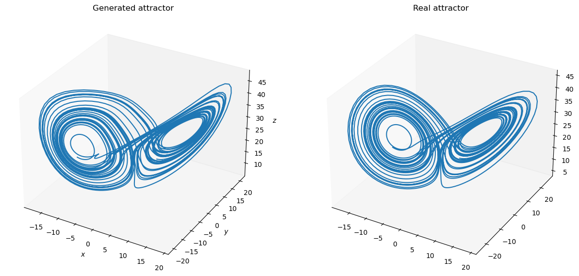
Here, we use ridge regression as the training algorithm to train the chaotic model.

trainer = bp.OfflineTrainer(model, fit_method=bp.algorithms.RidgeRegression(1e-7), dt=dt)

# first warmup the reservoir

_ = trainer.predict(X_warmup)

# then fit the reservoir model

_ = trainer.fit([X_train, Y_train])

def plot_lorenz(ground_truth, predictions):
  fig = plt.figure(figsize=(15, 10))
  ax = fig.add_subplot(121, projection='3d')
  ax.set_title("Generated attractor")
  ax.set_xlabel("$x$")
  ax.set_ylabel("$y$")
  ax.set_zlabel("$z$")
  ax.grid(False)
  ax.plot(predictions[:, 0], predictions[:, 1], predictions[:, 2])

  ax2 = fig.add_subplot(122, projection='3d')
  ax2.set_title("Real attractor")
  ax2.grid(False)
  ax2.plot(ground_truth[:, 0], ground_truth[:, 1], ground_truth[:, 2])
  plt.show()

# finally, predict the model with the test data

outputs = trainer.predict(X_test)
print('Prediction NMS: ', bp.losses.mean_squared_error(outputs, Y_test))
plot_lorenz(bm.as_numpy(Y_test).squeeze(), bm.as_numpy(outputs).squeeze())

Prediction NMS:  0.858903742335844

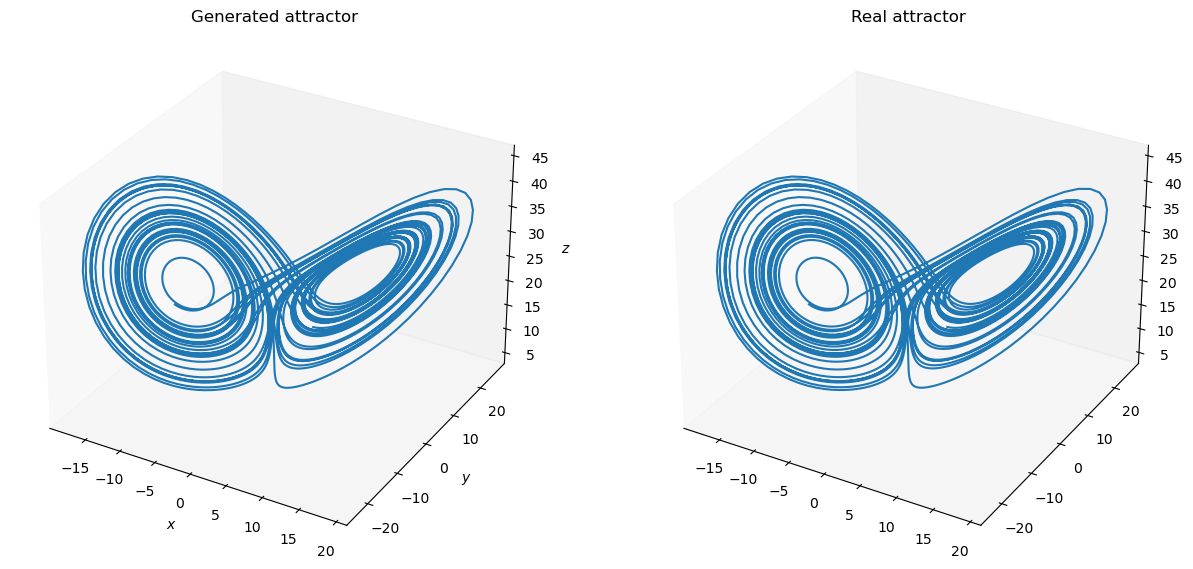
Switch different training algorithms

brainpy.OfflineTrainer supports easy switch of training algorithms. You just need provide the fit_method argument when instantiating an offline trainer.

Many offline algorithms, like linear regression, ridge regression, and Lasso regression, have been provided as the build-in models.

model = ESN(3, 100, 3)
model.reset(1)
trainer = bp.OfflineTrainer(model, fit_method=bp.algorithms.LinearRegression())

_ = trainer.predict(X_warmup)
_ = trainer.fit([X_train, Y_train])
outputs = trainer.predict(X_test)
plot_lorenz(bm.as_numpy(Y_test).squeeze(), bm.as_numpy(outputs).squeeze())

Customize your training algorithms

brainpy.OfflineTrainer also supports to train models with your customized training algorithms.

Specifically, the customization of an offline algorithm should follow the interface of brainpy.algorithms.OfflineAlgorithm, in which users specify how the model parameters are calculated according to the input, prediction, and target data.

For instance, here we use the Lasso model provided in scikit-learn package to define an offline training algorithm.

from sklearn.linear_model import Lasso

class LassoAlgorithm(bp.algorithms.OfflineAlgorithm):
  def __init__(self, alpha=1., max_iter=int(1e4)):
    super(LassoAlgorithm, self).__init__()
    self.model = Lasso(alpha=alpha, max_iter=max_iter)

  def __call__(self, y, x, outs=None):
    x = bm.as_numpy(x[0])
    y = bm.as_numpy(y[0])
    x_new = self.model.fit(x, y).coef_.T
    return bm.expand_dims(bm.asarray(x_new), 1)

model = ESN(3, 100, 3)
model.reset_state(1)

# note here scikit-learn algorithms does not support JAX jit,
# therefore the "jit" of the "fit" phase is set to be False.
trainer = bp.OfflineTrainer(model,
                            fit_method=bp.algorithms.LinearRegression(),
                            jit={'fit': False})

_ = trainer.predict(X_warmup)
_ = trainer.fit([X_train, Y_train])
outputs = trainer.predict(X_test)
plot_lorenz(bm.as_numpy(Y_test).squeeze(), bm.as_numpy(outputs).squeeze())