Customizing Your Neuron Models

@Xiaoyu Chen @Chaoming Wang

The previous section shows all available models users can utilize by simply instantiating the abstract model. In following sections we will dive into details to illustrate how to build a neuron model with brainpy.dyn.NeuDyn. Neurons are the most basic components in neural dynamics simulation. In BrainPy, brainpy.dyn.NeuDyn is used for neuron modeling.

import numpy as np

import brainpy as bp
import brainpy.math as bm

bm.set_platform('cpu')

bp.__version__

'2.4.4.post4'

brainpy.dyn.NeuDyn

Generally, any neuron model can evolve continuously or discontinuously. Discontinuous evolution may be triggered by events, such as the reset of membrane potential. Moreover, it is common in a neural system that a dynamical system has different states, such as the excitable or refractory state in a leaky integrate-and-fire (LIF) model. In this section, we will use two examples to illustrate how to capture these complexities in neuron modeling.

Defining a neuron model in BrainPy is simple. You just need to inherit from brainpy.dyn.NeuDyn, and satisfy the following two requirements:

• Providing the size of the neural group in the constructor when initialize a new neural group class. size can be a integer referring to the number of neurons or a tuple/list of integers referring to the geometry of the neural group in different dimensions. According to the provided group size, brainpy.dyn.NeuDyn will automatically calculate the total number num of neurons in this group.

• Creating an update() function. Update function provides the rule how the neuron states are evolved from the current time \(t\) to the next time \(t+dt\).

In the following part, a Hodgkin-Huxley (HH) model is used as an example for illustration.

Hodgkin–Huxley Model

The Hodgkin-Huxley (HH) model is a continuous-time dynamical system. It is one of the most successful mathematical models of a complex biological process that has ever been formulated. Changes of the membrane potential influence the conductance of different channels, elaborately modeling the neural activities in biological systems. Mathematically, the model is given by:

\[\begin{split} \begin{aligned} C_m \frac {dV} {dt} &= -(\bar{g}_{Na} m^3 h (V -E_{Na}) + \bar{g}_K n^4 (V-E_K) + g_{leak} (V - E_{leak})) + I(t) \quad\quad(1) \\ \frac {dx} {dt} &= \alpha_x (1-x) - \beta_x, \quad x\in {\rm{\{m, h, n\}}} \quad\quad(2) \\ &\alpha_m(V) = \frac {0.1(V+40)}{1-\exp(\frac{-(V + 40)} {10})} \quad\quad(3) \\ &\beta_m(V) = 4.0 \exp(\frac{-(V + 65)} {18}) \quad\quad(4) \\ &\alpha_h(V) = 0.07 \exp(\frac{-(V+65)}{20}) \quad\quad(5) \\ &\beta_h(V) = \frac 1 {1 + \exp(\frac{-(V + 35)} {10})} \quad\quad(6) \\ &\alpha_n(V) = \frac {0.01(V+55)}{1-\exp(-(V+55)/10)} \quad\quad(7) \\ &\beta_n(V) = 0.125 \exp(\frac{-(V + 65)} {80}) \quad\quad(8) \\ \end{aligned} \end{split}\]

where \(V\) is the membrane potential, \(C_m\) is the membrane capacitance per unit area, \(E_K\) and \(E_{Na}\) are the potassium and sodium reversal potentials, respectively, \(E_l\) is the leak reversal potential, \(\bar{g}_K\) and \(\bar{g}_{Na}\) are the potassium and sodium conductance per unit area, respectively, and \(\bar{g}_l\) is the leak conductance per unit area. Because the potassium and sodium channels are voltage-sensitive, according to the biological experiments, \(m\), \(n\) and \(h\) are used to simulate the activation of the channels. Specially, \(n\) measures the activation of potassium channels, and \(m\) and \(h\) measures the activation and inactivation of sodium channels, respectively. \(\alpha_{x}\) and \(\beta_{x}\) are rate constants for the ion channel x and depend exclusively on the membrane potential.

To implement the HH model, variables should be specified. According to the above equations, the following state variables change with respect to time:

• V: the membrane potential

• m: the activation of sodium channels

• h: the inactivation of sodium channels

• n: the activation of potassium channels

Besides, the spiking state and the last spiking time can also be recorded for statistic analysis:

• spike: whether a spike is produced

• t_last_spike: the last spiking time

Based on these state variables, the HH model can be implemented as below.

class HH(bp.dyn.NeuDyn):
  def __init__(self, size, ENa=50., gNa=120., EK=-77., gK=36., EL=-54.387, gL=0.03,
               V_th=20., C=1.0, **kwargs):
    # providing the group "size" information
    super(HH, self).__init__(size=size, **kwargs)

    # initialize parameters
    self.ENa = ENa
    self.EK = EK
    self.EL = EL
    self.gNa = gNa
    self.gK = gK
    self.gL = gL
    self.C = C
    self.V_th = V_th

    # initialize variables
    self.V = bm.Variable(bm.random.randn(self.num) - 70.)
    self.m = bm.Variable(0.5 * bm.ones(self.num))
    self.h = bm.Variable(0.6 * bm.ones(self.num))
    self.n = bm.Variable(0.32 * bm.ones(self.num))
    self.spike = bm.Variable(bm.zeros(self.num, dtype=bool))
    self.t_last_spike = bm.Variable(bm.ones(self.num) * -1e7)

    # integral functions
    self.int_V = bp.odeint(f=self.dV, method='exp_auto')
    self.int_m = bp.odeint(f=self.dm, method='exp_auto')
    self.int_h = bp.odeint(f=self.dh, method='exp_auto')
    self.int_n = bp.odeint(f=self.dn, method='exp_auto')

  def dV(self, V, t, m, h, n, Iext):
    I_Na = (self.gNa * m ** 3.0 * h) * (V - self.ENa)
    I_K = (self.gK * n ** 4.0) * (V - self.EK)
    I_leak = self.gL * (V - self.EL)
    dVdt = (- I_Na - I_K - I_leak + Iext) / self.C
    return dVdt

  def dm(self, m, t, V):
    alpha = 0.1 * (V + 40) / (1 - bm.exp(-(V + 40) / 10))
    beta = 4.0 * bm.exp(-(V + 65) / 18)
    dmdt = alpha * (1 - m) - beta * m
    return dmdt
  
  def dh(self, h, t, V):
    alpha = 0.07 * bm.exp(-(V + 65) / 20.)
    beta = 1 / (1 + bm.exp(-(V + 35) / 10))
    dhdt = alpha * (1 - h) - beta * h
    return dhdt

  def dn(self, n, t, V):
    alpha = 0.01 * (V + 55) / (1 - bm.exp(-(V + 55) / 10))
    beta = 0.125 * bm.exp(-(V + 65) / 80)
    dndt = alpha * (1 - n) - beta * n
    return dndt

  def update(self, x=None):
    _t = bp.share['t']
    _dt = bp.share['dt']
    x = 0. if x is None else x
    
    # compute V, m, h, n
    V = self.int_V(self.V, _t, self.m, self.h, self.n, x, dt=_dt)
    self.h.value = self.int_h(self.h, _t, self.V, dt=_dt)
    self.m.value = self.int_m(self.m, _t, self.V, dt=_dt)
    self.n.value = self.int_n(self.n, _t, self.V, dt=_dt)

    # update the spiking state and the last spiking time
    self.spike.value = bm.logical_and(self.V < self.V_th, V >= self.V_th)
    self.t_last_spike.value = bm.where(self.spike, _t, self.t_last_spike)

    # update V
    self.V.value = V

When defining the HH model, equation (1) is accomplished by brainpy.odeint as an ODEIntegrator. The details are contained in the Numerical Solvers for ODEs tutorial.

The variables, which will be updated during dynamics simulation, should be packed as brainpy.math.Variable and thus can be processed by JIT compilers to accelerate simulation.

In the following part, a leaky integrate-and-fire (LIF) model is introduced as another example for illustration.

Leaky Integrate-and-Fire Model

The LIF model is the classical neuron model which contains a continuous process and a discontinous spike reset operation. Formally, it is given by:

\[\begin{split} \begin{aligned} \tau_m \frac{dV}{dt} = - (V(t) - V_{rest}) + I(t) \quad\quad (1) \\ \text{if} \, V(t) \gt V_{th}, V(t) =V_{rest} \, \text{after} \, \tau_{ref} \, \text{ms} \quad\quad (2) \end{aligned} \end{split}\]

where \(V\) is the membrane potential, \(V_{rest}\) is the rest membrane potential, \(V_{th}\) is the spike threshold, \(\tau_m\) is the time constant, \(\tau_{ref}\) is the refractory time period, and \(I\) is the time-variant synaptic inputs.

The above two equations model the continuous change and the spiking of neurons, respectively. Moreover, it has multiple states: subthreshold state, and spiking or refractory state. The membrane potential \(V\) is integrated according to equation (1) when it is below \(V_{th}\). Once \(V\) reaches the threshold \(V_{th}\), according to equation (2), \(V\) is reaet to \(V_{rest}\), and the neuron enters the refractory period where the membrane potential \(V\) will remain constant in the following \(\tau_{ref}\) ms.

The neuronal variables, like the membrane potential and external input, can be captured by the following one variable:

• V: the membrane potential

In order to define the different states of a LIF neuron, we define additional variables:

• spike: whether a spike is produced

• refractory: whether the neuron is in the refractory period

• t_last_spike: the last spiking time

Based on these state variables, the LIF model can be implemented as below.

class LIF(bp.dyn.NeuDyn):
  def __init__(self, size, V_rest=0., V_reset=-5., V_th=20., R=1., tau=10., t_ref=5., **kwargs):
    super(LIF, self).__init__(size=size, **kwargs)

    # initialize parameters
    self.V_rest = V_rest
    self.V_reset = V_reset
    self.V_th = V_th
    self.R = R
    self.tau = tau
    self.t_ref = t_ref

    # initialize variables
    self.V = bm.Variable(bm.random.randn(self.num) + V_reset)
    self.t_last_spike = bm.Variable(bm.ones(self.num) * -1e7)
    self.refractory = bm.Variable(bm.zeros(self.num, dtype=bool))
    self.spike = bm.Variable(bm.zeros(self.num, dtype=bool))

    # integral function
    self.integral = bp.odeint(f=self.derivative, method='exp_auto')

  def derivative(self, V, t, Iext):
    dvdt = (-V + self.V_rest + self.R * Iext) / self.tau
    return dvdt

  def update(self, x=None):
    _t = bp.share['t']
    _dt = bp.share['dt']
    x = 0. if x is None else x
    
    # Whether the neurons are in the refractory period
    refractory = (_t - self.t_last_spike) <= self.t_ref
    
    # compute the membrane potential
    V = self.integral(self.V, _t, x, dt=_dt)
    
    # computed membrane potential is valid only when the neuron is not in the refractory period 
    V = bm.where(refractory, self.V, V)
    
    # update the spiking state
    spike = self.V_th <= V
    self.spike.value = spike
    
    # update the last spiking time
    self.t_last_spike.value = bm.where(spike, _t, self.t_last_spike)
    
    # update the membrane potential and reset spiked neurons
    self.V.value = bm.where(spike, self.V_reset, V)
    
    # update the refractory state
    self.refractory.value = bm.logical_or(refractory, spike)

In above, the discontinous resetting is implemented with brainpy.math.where operation.

Instantiation and running

Here, let’s try to instantiate a HH neuron group:

neu = HH(10)

in which a neural group containing 10 HH neurons is generated.

In brief, running any dynamical system instance should be accomplished with a runner, such like brianpy.DSRunner. The variables to be monitored and the input crrents to be applied in the simulation can be provided when initializing the runner.

runner = bp.DSRunner(neu, monitors=['V'])

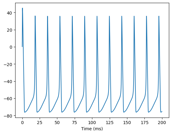
At each time step, we give the same input current:

inputs = np.ones(int(200. / bm.get_dt())) * 6.  # 200 ms

Then the simulation can be performed with a given time period, and the simulation result can be visualized:

runner.run(inputs=inputs)  # the running time is 200 ms

bp.visualize.line_plot(runner.mon.ts, runner.mon.V, show=True)

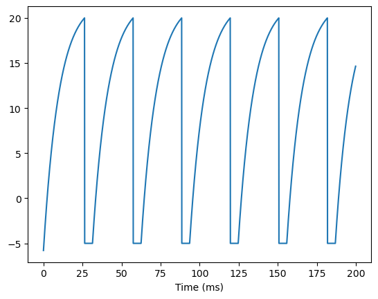
A LIF neural group can be instantiated and applied in simulation in a similar way:

group = LIF(10)

runner = bp.DSRunner(group, monitors=['V'])

inputs = np.ones(int(200. / bm.get_dt())) * 22.  # 200 ms
runner.run(inputs=inputs)

bp.visualize.line_plot(runner.mon.ts, runner.mon.V, show=True)