AMPA#
- class brainpy.dyn.AMPA(size, keep_size=False, sharding=None, method='exp_auto', name=None, mode=None, alpha=0.98, beta=0.18, T=0.5, T_dur=0.5)[source]#
AMPA synapse model.
Model Descriptions
AMPA receptor is an ionotropic receptor, which is an ion channel. When it is bound by neurotransmitters, it will immediately open the ion channel, causing the change of membrane potential of postsynaptic neurons.
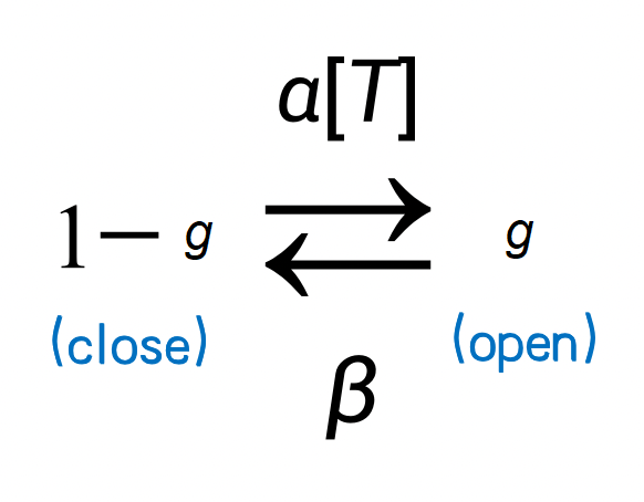
A classical model is to use the Markov process to model ion channel switch. Here \(g\) represents the probability of channel opening, \(1-g\) represents the probability of ion channel closing, and \(\alpha\) and \(\beta\) are the transition probability. Because neurotransmitters can open ion channels, the transfer probability from \(1-g\) to \(g\) is affected by the concentration of neurotransmitters. We denote the concentration of neurotransmitters as \([T]\) and get the following Markov process.
We obtained the following formula when describing the process by a differential equation.
\[\frac{ds}{dt} =\alpha[T](1-g)-\beta g\]where \(\alpha [T]\) denotes the transition probability from state \((1-g)\) to state \((g)\); and \(\beta\) represents the transition probability of the other direction. \(\alpha\) is the binding constant. \(\beta\) is the unbinding constant. \([T]\) is the neurotransmitter concentration, and has the duration of 0.5 ms.
Moreover, the post-synaptic current on the post-synaptic neuron is formulated as
\[I_{syn} = g_{max} g (V-E)\]where \(g_{max}\) is the maximum conductance, and E is the reverse potential.
This module can be used with interface
brainpy.dyn.ProjAlignPreMg2, as shown in the following example:import numpy as np import brainpy as bp import brainpy.math as bm import matplotlib.pyplot as plt class AMPA(bp.Projection): def __init__(self, pre, post, delay, prob, g_max, E=0.): super().__init__() self.proj = bp.dyn.ProjAlignPreMg2( pre=pre, delay=delay, syn=bp.dyn.AMPA.desc(pre.num, alpha=0.98, beta=0.18, T=0.5, T_dur=0.5), comm=bp.dnn.CSRLinear(bp.conn.FixedProb(prob, pre=pre.num, post=post.num), g_max), out=bp.dyn.COBA(E=E), post=post, ) class SimpleNet(bp.DynSysGroup): def __init__(self, E=0.): super().__init__() self.pre = bp.dyn.SpikeTimeGroup(1, indices=(0, 0, 0, 0), times=(10., 30., 50., 70.)) self.post = bp.dyn.LifRef(1, V_rest=-60., V_th=-50., V_reset=-60., tau=20., tau_ref=5., V_initializer=bp.init.Constant(-60.)) self.syn = AMPA(self.pre, self.post, delay=None, prob=1., g_max=1., E=E) def update(self): self.pre() self.syn() self.post() # monitor the following variables conductance = self.syn.proj.refs['syn'].g current = self.post.sum_inputs(self.post.V) return conductance, current, self.post.V indices = np.arange(1000) # 100 ms, dt= 0.1 ms conductances, currents, potentials = bm.for_loop(SimpleNet(E=0.).step_run, indices, progress_bar=True) ts = indices * bm.get_dt() fig, gs = bp.visualize.get_figure(1, 3, 3.5, 4) fig.add_subplot(gs[0, 0]) plt.plot(ts, conductances) plt.title('Syn conductance') fig.add_subplot(gs[0, 1]) plt.plot(ts, currents) plt.title('Syn current') fig.add_subplot(gs[0, 2]) plt.plot(ts, potentials) plt.title('Post V') plt.show()
- Parameters:
alpha (
Union[float,TypeVar(ArrayType,Array,Variable,TrainVar,Array,ndarray),Callable]) – float, ArrayType, Callable. Binding constant.beta (
Union[float,TypeVar(ArrayType,Array,Variable,TrainVar,Array,ndarray),Callable]) – float, ArrayType, Callable. Unbinding constant.T (
Union[float,TypeVar(ArrayType,Array,Variable,TrainVar,Array,ndarray),Callable]) – float, ArrayType, Callable. Transmitter concentration when synapse is triggered by a pre-synaptic spike.. Default 1 [mM].T_dur (
Union[float,TypeVar(ArrayType,Array,Variable,TrainVar,Array,ndarray),Callable]) – float, ArrayType, Callable. Transmitter concentration duration time after being triggered. Default 1 [ms]size (
Union[int,Sequence[int]]) – int, or sequence of int. The neuronal population size.keep_size (
bool) – bool. Keep the neuron group size.
- supported_modes: Optional[Sequence[bm.Mode]] = (<class 'brainpy._src.math.modes.NonBatchingMode'>, <class 'brainpy._src.math.modes.BatchingMode'>)#
Supported computing modes.